the Tokamaks, and by a reversed toroidal field in the vacuum region outside the plasma. Since the beginning of the RFX operation the wall locked modes had ...
A neural network approach for the detection of the locking position in RFX O. Barana, G. Manduchi, A. Serri*, P.Sonato* Consorzio RFX Corso Stati Uniti 4, I-35127 PADOVA (Italy) *Dipartimento di Ingegneria Elettrica ed Elettronica,Università di Cagliari Piazza d’Armi, I-09123 CAGLIARI (ITALY) Abstract - Recently in RFX, where wall locked modes were always present, a new technique has demonstrated the possibility to induce a continuous rotation of the modes with respect to the wall. In this technique the non-linear coupling of the m=0 and m=1 modes has been used to decouple the modes themselves. In the present experiments the mode rotation is induced with a preprogrammed waveform of a toroidal magnetic field rotating ripple. A feedback system able to create a continuous rotation with variable and increasing speed is now under implementation. A Neural Network (NN) has been developed to identify the locked mode position. In the paper different NNs are presented, discussed and compared. I. - INTRODUCTION RFX (Reversed Field eXperiment) is one of the three major RFP (Reversed Field Pinch) operating devices in the fusion community. The RFP magnetic configuration is characterized by a low toroidal field, in comparison with the Tokamaks, and by a reversed toroidal field in the vacuum region outside the plasma. Since the beginning of the RFX operation the wall locked modes had always been present during the whole reversed toroidal field phase of the discharge [1]. The presence of locked modes has been proven in all the other major RFP experiments: MST [2] and TPE-RX [3]. The presence of modes that are locked in phase induces the breaking of the plasma toroidal symmetry and consequently a concentrated plasma column Localized Helical Deformation (LHD) appears having a toroidal extension of approximately 40° [1]. The LHD is due to the locking in phase of the MHD resonant modes with a characteristic spectrum m=1 and n=7-12 [1,8]. This locking in phase of tearing modes and the possibility to control the phenomenon is of great significance not only for the RFP experiments but also for the Tokamaks because the LHD induces an increased and uncontrolled plasma wall interaction with, at least, a degradation of the plasma performance and a possible damage of the first wall components [4]. Recently in RFX a new technique has demonstrated the possibility to unlock the modes with respect to each other and also with respect to the wall [5,6]. A continuous rotation of the LHD has been induced with a preprogrammed waveform of a rotating ripple of the toroidal magnetic field that mainly produces an m=0, n=1 rotating mode [6,7]. The externally induced m=0, n=1 mode is able to drag the m=0 n=1 mode associated with the
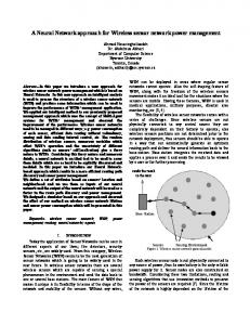
LHD in the plasma and, through the non-linear coupling between the m=0 and the m=1 modes in the plasma itself, the m=1 modes starts to rotate [8]. An electromagnetic synchronous torque is applied by the m=0, n=1 external mode on the plasma m=0 n=1 mode [8]. This torque is contrasted by the torque due to the static and dynamic error fields, the plasma viscosity and the eddy currents induced in the passive structures that surround the plasma column [8]. This braking torque is obviously depending on the magnetic configuration control and on many plasma parameters. A feedback system able to detect the LHD position along the toroidal coordinate and able to create a continuous rotation with variable speed is therefore envisaged to overcome the identified but unknown contrasting torque. The feedback system should control the synchronization between the m=0, n=1 external rotating toroidal field ripple and the m=0, n=1 plasma mode which is associated to the LHD. II. - THE IDENTIFICATION OF LHD POSITION The LHD position is identified after the shots by means of Fourier Analysis of the toroidal magnetic field acquired from two arrays of 72 electromagnetic pick up coils uniformly distributed along the torus. In fig.1 the temporal evolution of the toroidal magnetic field odd part around the torus is shown for the shot 13228. The figure clearly shows the presence of the non-axisymmetric toroidal field in a portion of the plasma column corresponding to the presence of the LHD. In figure 2 it is shown the calculated LHD position for the same shot. Due to required computation time, it would not be possible to retrieve the LHD position “on the flight” during the pulse, and therefore alternative approaches, based on the Neural Networks (NN) have been investigated. Fast detection of the LHD position is in fact required in an implementation of a feedback control system that could control the position of the LHD. III. - THE NEURAL NETWORK APPROACH The NN approach for the detection problem of the LHD position, as well as any other functional dependence problem, allows to avoid direct mathematical modeling of the system behavior. A neural network is a parallel system constituted by units (neurons) with multiple connections (thus resulting in a network). Each neuron is an elementary computation unit that outputs a single value depending on the value of its inputs (activation function). NN architecture specifies the
LHD toroidal position
0.1
time (s)
0.08 0.06 0.04 0.02 0 0
40
80
120 160 200 240 280 320 360 toroidal angle Fig.1 The odd part of the toroidal magnetic field in the shot #13228.
360 320 280 240 200 160 120 80 40 00
0.02
0.04
0.06 0.08 0.1 0.12 time (s) Fig.2 The calculated LHD position for the shot #13228
layout of its units, their activation functions and their connections. The term of artificial NN addresses the ability at learning by examples. Artificial neural networks are powerful computation tools that can reproduce the desired input-output relationship starting from an adequate number of examples. There is a lot of literature dealing with artificial intelligence and neural networks, but it is useful to give here only a simple description of the specific application avoiding theoretical details [9]. Briefly, starting from an adequate network architecture, good training data (examples) should be supplied to evaluate the most suited training algorithm. Each example consists of an input pattern and the corresponding (desired) output. In our application, input patterns are represented by the odd part of the toroidal magnetic field, sampled at 69 available different angular positions, and the output represents the angular position of the LHD. The NN resulting from this schedule has to be tested to check for possible improvements regarding architecture, training set and learning algorithm. Roughly speaking, a trial and error procedure must be adopted. First of all, let us assume that it is possible to state the detection problem as a time-indepedent and memoryless relationship between the magnetic measures and the locked-mode position: Position = f (toroidal field odd part: 69 inputs)
(1)
Under the above hypothesis, the function f of equation 1 should exist and, if it is monodrome, a feedforward Multi Layer Perceptron neural network (MLP) can approximate it. MLP is particularly suitable thanks to the robustness of its training algorithm based on the so-called error back propagation. The MLP is completely identified by giving the number of layers, the number of units for each layer and the values of the connection strengths (weights). In addition MLP requires one or two hidden layers with a number of units that can be related to the complexity of the desired input-output relationship. Figure 3 shows the general architecture of the MLP with input, output and at least one hidden layer. Weights may be identified for each layer (except from the input layer) by using the indexes of the connected units. Moreover proper bias for each unit may be considered as an additional input of constant value connected to all the network units. For our neural estimator, the input layer has 69 different values that will be passed to the units of the subsequent layer using different weights. To completely define the architecture of the neural estimator, an adequate number of hidden units must be chosen. These hidden units may be arranged in a single hidden layer or in multiple hidden layers affecting only the performances of the training algorithm. All units of the NN have symmetrical saturating activation function very close to the hyperbolic tangent function. The chosen NN is completely known when the values of weights and biases are defined. The training algorithm allows for optimal determination of these values with respect to the overall squared error. Thus, it is evident that
Fi g.3 Gene ar l archi ec t ure t of a ne ura lnetwo kr
the input-output patterns for training are to be carefully selected. The robustness of MLP allows to reduce the effect of few bad data in the training set. Magnetic data derive from 45 different shots and their corresponding LHD positions computed from off-line algorithm have been selected. Considering the sampling time, about 80000 patterns were available for learning. Part of this set has been used for the training, and the remaining patterns have been used to test the trained NN. IV. – NEURAL NETWORK ARCHITECTURES Two different network architectures implying two different approaches of the output units have been tested for the detection of the angular position of the LHD. Continuous estimator NN approach (Cont-NN) In the first one the NN is trained to directly generate the angular position of the LHD. However direct use of equation (1) is dangerous due to the discontinuity in position values. In the relevant application, position value spans from 0° to 360° and these extreme values represent the same physical condition, thus function f results double determined. Further considerations about function continuity and neural approximation lead us to locate the position α as the couple of two values: sin(α) and cos(α). Consequently, using this approach, the MLP has an output layer which consists of two units. The number of hidden units in the MLP plays an important role in the ability of the NN at adequately model the desired transfer function. Table I lists the performances with different numbers of hidden units for three different test sets: the training set (5000 patterns), the original set (Test I) of 80.000 patterns taken from the same shots, and a third set (Test II) of 30.000 new patterns, taken from different shots. To represent performance, two error classes are presented in each column for each set. The left one is characterized by an estimation error less than 1/12 (i.e. ± 1/24) of round, while the right one is characterized by an estimation error less than 1/6 (i.e. ± 1/12) of round. The numbers in the table represent the percentage of correct identifications (i.e. within the corresponding error). Table I Continuous estimator NN performance N° of hidden units
Test II [%]
Training results [%]
Test I [%]
5
42
65
53
77
26
47
6
54
78
45
71
37
57
10
77
93
74
91
50
69
15
74
91
70
88
52
73
20
79
92
75
90
54
75
The results in Table I show that increasing the number of the network units, the learning capability increases, making however proper generalization more difficult to achieve. It has also been checked that the input pattern variation corresponding to a small range of position is wide. Thus, many iterations of the training algorithm are not effective and “early stopping“ technique is most suitable. Moreover, large NN may result not efficient when considering the on-line requirements. In conclusion the NN with 15 hidden neurons may represent a good trade-off, while larger NNs result in negligible performance improvement. In figure 4 it is shown, for a test shot #13228 (not used for the training), the comparison between the calculated LHD position (dotted line) and the continuous estimator NN (Cont-NN) estimated position (solid line). In figure 5 it is shown the difference between the two quantities, where it is evident that, for the whole shot duration, the angular difference is lower than 40° except for the jumping position at 360°.
0
0.02
toroidal coordinate
calculated Cont-NN
toroidal coordinate
360 320 280 240 200 160 120 80 40 0
calculated C-NN
0.06 0.08 0.1 0.12 time (s) Fig.6 Result of the Classifier NN (C-NN) compared with the calculated LHD position for the shot #13228
0.04
0.06 0.08 0.1 0.12 time (s) Fig.4 Result of the continuous estimation NN (Cont-NN) compared with the calculated LHD position for the shot #13228
80
0
0.02
0.04
0
0.02
0.04
angular difference
80
40 0
-40 -80 0
0.02
0.04
0.06 0.08 0.1 0.12 time (s) Fig.5 Angular difference between Cont-NN and calculated LHD position for the shot #13228
Classifier NN approach (C-NN) In the second approach a MLP is still used, but the angular position identification problem of the LHD perturbation is seen as a classification problem, where each class represents the index in a set of 12 discretized angular positions. The reason for this choice derives from the fact that the number of classes is the number of the toroidal winding sectors (12 toroidal winding sectors in RFX), and a control system needs to identify which coil is located closest to LHD position. In classification problems, an 1 to N approach is usually adopted, where the NN is defined with a number of output units which is equal to the number of classes, and is trained to generate a value of 1 in the output unit corresponding to the input class, and 0 in all other output units. When trained, the network is used as a classifier by selecting the output with the highest activation as the representative of the class of the input pattern. It is proved that, in the ideal condition in which the network has an unbounded plasticity, it behaves like a Bayesan classifier which minimizes the probability of misclassification [10]. However, in real cases, better results are achieved using a smoother activation shape for the output units by training the network to produce a set of outputs representing the sampled values of a gaussian function centered at the desired position. As in the conventional approach, after the network has been trained, the (discretized) angular position of the locking is determined by the output units with the highest activation. In figure 6 it is shown, for the test shot #13228 (not used for the training), the comparison between the calculated LHD position (dotted line) and the classifier NN (C-NN) estimated position (solid line). In figure 7 it is shown the difference between the two quantities, where it is evident that, for the whole, shot duration, the angular difference is lower than 40° except for the jumping position at 360°. It is then possible to define an optimal width of the gaussian form which maximize the probability of correct classification. Figure 8 shows the probability of having a correct classification versus the width (sigma) of the gaussian activation form for a set of 30000 pattern (Test Set II of Table I).
40 0 -40 -80 0.06 0.08 0.1 0.12 time (s) Fig.7 Angular difference between C-NN and calculated LHD position for the shot #13228
Self-check of quality estimation Using both approaches, a quality factor can be derived from the output of the NN, giving an indication about the reliability of the current result. This information is important when implementing a control system in order to avoid a wrong detection of the angular position of the LHD. The possibility of deriving a quality factor is a consequence of the well known limited ability of NNs in extrapolation. Consequently, an input pattern not belonging to the space defined by the training set will produce an unpredictable output. Therefore, if the input to the trained NNs does not define a LHD position (e.g. when input patterns exhibit no locked-mode or exhibit quasi single helicity therefore no control action is required), the output activation of the NN will be unlikely to have the expected form. In the first approach this 2corresponds to the check of 2 the identity 1=sin(α) +cos(α) on the two NN outputs (fig.9). In the second approach the quality factor is based on the mean square difference between an exact gaussian function centered at the position corresponding to the output unit with the maximum activation, and the actual network outputs (fig.10). 90 classification rate (%)
angular difference
360 320 280 240 200 160 120 80 40 0
85 80 75 70 0
1
2 3 4 5 gaussian width (sigma) Fig.8 Classification rate probability versus the gaussian activation sigma width
6
the correlation parameter is lower than 0.8 are fewer than 5% of the total test set. The obtained results, together with the possibility of controlling the toroidal field winding sectors having an extension of 30°, show the sufficient reliability and robustness of the chosen approach.
2 1.5
VI. - CONCLUSION
1 0.5 00
0.02
0.04
0.06 0.08 0.1 0.12 time (s) 2 2 Fig.9 (sen +cos ) output parameter evaluated for the two output of Cont-NN for the shot #13228
quality factor (a.u.)
1.4 1.2 1 0.8 0.6 0.4 0.2 00
0.02
0.04
0.06 0.08 0.1 0.12 time (s) Fig.10 Quality factor in the C-NN for the shot #13228
It is therefore possible in both cases to define a threshold in the quality factor, in order to discriminate between “good” measurements (i.e. for which the computation of the locking is assumed to be valid) and “bad” ones. V. – COMPARISON The efficiency of the two NNs has been verified on a test set of 90 shots. The test set has been chosen with a wide range of plasma current between 500 kA and 1.2 MA. In the set have been included two different classes of shots: shots with externally induced mode rotation and shots without externally induced mode rotation. Some shots have been also included where a fast rotated toroidal ripple (frequency > 100 Hz) was produced. Finally a subset of shots was considered where the LHD seems to vanish on a significant portion of the discharge and some shots where it is present the so called Quasi Single Helicity (QSH) state characterized by a single dominant mode, normally m=1 n=8 (but sometimes also n=7 or n=9). In this situation the plasma assumes a complete helical toroidal shape without any LHD. This last two subset of examples have been included because they represent a very recent magnetic configuration that has not been used to train the NNs and where the algorithm to calculate the LHD position is meaningless. A correlation parameter has been identified to evaluate the coincidence between the calculated LHD position and the NNs output: this parameter is derived from the weighted mean of the difference between the NN output and the calculated LHD position over the whole shot duration. When the difference is 0 for the whole shot duration then the value of this parameter is 1. In figure 11 it is shown the percentage distribution of the correlation parameter for all the shots included in the test set. It is evident that for both the NNs more than 65% of the shots have a correlation parameter greater that 0.9. This means that the mean difference between the NN result and the calculated LHD position differs less than 20° in the toroidal position for the whole pulse. Furthermore, 90% of the shots show a correlation parameter greater than 80%: this means a difference of less than 40° in the toroidal position of the LHD identification. Finally, the shots where
A satisfactory identification of the LHD has been reached with two different Neural Networks architectures. In the next scheduled shutdown the two NNs will be implemented on the RFX digital control system, as a feedback signal to control the rotation of the LHD position i.e. to control the rotation of the wall locked modes. REFERENCES [1] A.Buffa, et al., "Magnetic field configurationst and locked modes in RFX", Proceedings of the 21 EPS Conference on Plasma Physics and Controlled Fusion, European Physical Society, vol.1, 1994, p.458-461. [2] A.F. Almagri, S. Assadi, S.C. Prager, J.S. Sarff, D.W. Kerst, “Locked modes and magnetic field errors in the Madison Symmetric Torus”, Physics of Fluids B, Vol.4, n.12, 1992, p.4080-4085. [3] Y.Yagi, et al., “The first results of TPE-RX, a large reversed-field pinch machine”, Plasma Physics and Controlled Fusion Vol.41, 1999, p.255–263. [4] P.Sonato, P.Zaccaria, "Thermal fluxes due to plasmawall interactions: experimental measurements and numerical analyses", Fusion Engineering and Design , Vol.39-40, 1998, p.401-408. [5] R.Piovan, “New power supply to generate a rotatingth toroidal field in RFX”, Proceedings of the 20 Symposium on Fusion Technology, Vol.1, 1998, p.853-856. [6] G.Chitarin, R.Piovan, P.Sonato, G.Zollino, “Control of thlocked mode position in RFX”, Proceedings of the 25 EPS Conference on Plasma Physics and Controlled Fusion, European Physical Society, 1998, p.766-769. [7] G.Zollino, “Diffusion of a rotating magnetic field through the RFX shell and vacuum vessel”, presented at Intermag99, Kyongju (Korea), 1999, to be published on the IEEE Trans. on Magnetics. [8] R.Bartiromo, et al., “Tearing mode rotation by external field in a reversed field pinch”, Physical Review Letters, Vol. 83, n.9, 1999, p.1779-1782. [9] J.Herz, A.Krog, R.G.Palmer, “Introduction to the theory of neural computation”, Addison Wesley, 1991. [10] D.W.Ruck, S.K.Rogers, M.Kabrisky, M.E.Oxley, B.W.Suter, “The multilayer perceptrons as an approximation to a Bayes optimal discriminant function”, IEEE Trans. on Neural Network, Vol.1, n.4, 1990, p.296-298.
70 shot percentage (%)
quality factor (a.u.)
2.5
60
Classifier-NN Continuous-NN
50 40 30 20 10 0
0.1 0.2 0.3 0.4 0.5 0.6 0.7 0.8 0.9 correlation factor (a.u.)
Fig.11 Correlation between the calculated LHD position and the two NNs for a test set of 90 shots
1