A Neural Network Approach to Condition Based ... - CiteSeerX

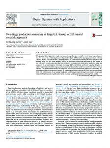
A Neural Network Approach to Condition Based Maintenance: Case Study of Airport Ground Transportation Vehicles Alice E. Smith Department of Industrial and Systems Engineering 207 Dunstan Hall Auburn University Auburn, AL 36849 USA David W. Coit Department of Industrial and Systems Engineering 96 Frelinghuysen Road Rutgers University Piscataway, NJ 08854 USA Yun-Chia Liang Department of Industrial Engineering Yuan Ze University Taoyuan, Taiwan Abstract This paper describes a joint industry/university collaboration to develop a prototype system to provide real time monitoring of an airport ground transportation vehicle with the objectives of improving availability and minimizing field failures by estimating the proper timing for condition-based maintenance. Hardware for the vehicle was designed, developed and tested to monitor door characteristics (voltage and current through the motor that opens and closes the doors and door movement time and position), to quickly predict degraded performance, and to anticipate failures. A combined statistical and neural network approach was implemented. The neural network “learns” the differences among door sets and can be tuned quite easily through this learning. Signals are processed in real time and combined with previous monitoring data to estimate, using the neural network, the condition of the door set relative to maintenance needs. The prototype system was installed on several vehicle door sets at the Pittsburgh International Airport and successfully tested for several months under simulated and actual operating conditions. Preliminary results indicate that improved operational reliability and availability can be achieved. Keywords: Condition monitoring, Conditional maintenance, Predictive maintenance, Preventive maintenance, Neural network, Transportation 1. Introduction Ground transportation people mover vehicles are found in every major airport in the world. These vehicles have stringent availability and safety demands. Although they operate over short, fixed routes, they are subject to nearly constant use, sometimes under adverse outdoors environments, with frequent stops and a large volume of passengers. One of the world’s leading producer of these systems, in cooperation with the University of Pittsburgh, and Auburn University, researched a proof

of concept for utilizing a condition-based maintenance approach for improving the operational reliability and availability of the vehicle door systems. Door systems were monitored in real time with respect to their current operational state and predictive models were developed to suggest when maintenance actions are required. The benefits anticipated using condition-based maintenance over the current scheduled maintenance approach are: 1) more cost effective maintenance because system and/or components are maintained only where and when needed and 2) degradation-type failures and downtime reduced to a minimum because systems and their components can be maintained during an early phase of degradation, long before failure can occur. The door system has the greatest need for maintenance at the people mover system sites and is a major factor impacting the availability of the transit system. Failure in the door system may force the people mover to be temporarily shut down due to safety concerns. Because of passengers holding the doors open, numerous open/close cycles and harsh weather conditions, the door’s system components are subject to a large amount of stress and deterioration. Deterioration in either the electrical DC motor that controls the operation of the door or the mechanical levers, rollers, tracks, or switches can cause failures in the subsystem. Currently, a labor-intensive preventive maintenance program is used to ensure high availability. This scheduled maintenance approach requires experienced personnel to determine the cause(s) of the problems and can result in components being serviced even though there is no need for maintenance. In summary, the door system was selected to implement and test the condition-based maintenance approach because it experiences a large number of degradation failures, it is fairly readily instrumented for monitoring and it has a very similar design over all models of the people mover vehicle line. Although an analytic model was considered and developed early in the project based on physicsof-failure concepts, it was not practical or effective. The analytic model could not account for all of the aspects of operation of a real people mover door set. Therefore, an empirical approach was used to process the signals from the people mover and estimate when maintenance should be performed. Because of the anticipated nonlinear behavior of the door system, neural networks were chosen as the primary predictive modeling tool. The appendix shows a flow chart of the monitoring and prediction system for condition based maintenance. Predictive maintenance and integrated prognostics involves condition monitoring, fault detection and prediction of future failures.

Degradation models can be used so that reliability

assessments can be made and updated based on observed degradation paths. Prognostics can be

1

defined as the capability to provide early detection and isolation of precursor and/or incipient fault condition to a component failure condition, and to have the means to manage and predict the progression of this fault condition to component failure. Significant research has been conducted on condition monitoring and integrated prognostics. El-Wardany et al. (1996) presented a study on condition monitoring of tool wear and failure in drilling operation using vibration signature analysis techniques; Szecsi (1999) demonstrated a cutting tool condition monitoring system for CNC lathes. The system is based on the measurement of the main DC motor current of the lathes. The system alarms when the cutting tool wear exceeds a predefined value. The monitoring system is trained by genetic algorithm and fuzzy logic based machine learning techniques; Dimla Jr. et al. (1997) presented a comprehensive review of tool condition monitoring systems, developed or implemented through application of neural networks; Prickett and Johns (1999) provided an overview of approaches to the detection of cutting tool wear and breakage during the milling process. Lu et al. (2001) developed a technique for predicting individual system performance reliability in real-time considering multiple failure modes.

This technique includes on-line multivariate

monitoring and forecasting of performance measures and conditional performance reliability estimates. The performance measures are treated as a multivariate time series and a state-space approach is used to model the multivariate time series. The predicted mean vectors and covariance matrix of performance measures are used for the assessment of system reliability. This technique provides a means to forecast and evaluate the performance degradation of an individual system in a dynamic environment in real-time. Greitzer et al. (1999) discussed a prototype monitoring and prognostic system for gas turbine engines. Artificial neural networks, rule-based algorithms, and predictive trend analysis tools were used to diagnose and predict engine conditions. Roemer and Kacprzynski (2000) described some novel diagnostic and prognostic technologies for gas turbine engine risk assessment. They presented an integrated set of turbo machinery condition monitoring, diagnostic and prognostic technologies. These technologies can be implemented across the entire spectrum of turbo machines from mid-sized pumps to land-based gas and steam engines as well as aircraft engines.

They claimed that

implementation of these technologies offers significant potential for reducing current product life cycle costs.

2

Neural networks have effectively been used in other applications to predict performance degradation of operating systems in real-time. Specifically, neural networks have been effective in anticipating failure for cutting tools (Choudhury et al., 1999, Das et al., 1997, Quan et al., 1998) and machinery (Chow et al., 1991, Lin and Wang, 1996). For these applications, sensors have been used to detect vibration and other effects of wear and to input into a trained neural network model. Additionally, there have been other applications including mining (Sottile and Holloway, 1994), hydro-electric power plants (Isasi et al., 2000) and component placement for surface mount technology (May et al., 1998). 2. Door System Description The door system operates as an open-loop system receiving signals from an automatic train control system that initiates opening or closing of the motor. The motor turns an operator arm, which runs along a guidance slot in the door (see Figure 1). The movement of the operator arm pulls or pushes the door to the open and closed positions. The door is equipped with rollers that ride in a track at the top of the vehicle and there is a track at the bottom of the vehicle in which the door rides. As the door goes through its cycle, micro-switches connect and disconnect resistors in the electrical circuitry, which change the speed of the moving door. The door typically opens in 3 to 3.5 seconds, and closes in 4 to 4.5 seconds.

Top Rollers and Track

Operator Arm Guidance Track

Operator Arm

Motor

Lower Track

Figure 1. Diagram of the door system. The available signals from the doors are time, current and voltage of each door leaf as it passes through a set of five switches. It is easy to calculate energy from the latter two, therefore the signals used were time and energy. Door position, while of potential value, cannot be readily monitored.

3

However, energy and timing can sufficiently characterize the condition of the door regarding degradation caused by contaminants in the track, track warping, engine wear out, etc. 3. Data Acquisition 3.1 On board data collection Because neural networks are data driven models, data under a variety of conditions needed to be obtained. Although it would have been useful to monitor some operating people movers in the field, there were practical restrictions that prevented this type of data collection. First, because of the public nature of airports, any alteration to a vehicle, even in the form of passive monitoring, is difficult to obtain approval for. Second, monitoring a field site does not allow control over the degradations or failures that might be experienced. Passive data collection from fielded systems may involve lengthy data collection intervals without significant degradation. Instead, an experimental set-up was made to gather data using a test vehicle provided by the industrial partner at their test track. The key measurable signals collected were the current through the motor, the voltage across the motor, the time interval of the open and close cycle, and the timing of the micro-switches. Using a sampling rate of 100 samples per second, all fluctuations in the data were easily detected. All signals pass through a circuit board that contains voltage dividers that scale down the voltage, and filters for the current measurements and motor voltage. The circuit board sends the signals to the built-in A/D converter, which, in turn, sends them to a laptop computer on-board. A software program was developed to compile the data in ASCII format. The data collection software was designed to collect data when both the closing voltage and the opening voltage are not equal to zero, i.e., data was only collected when the door system was in operation. Then, the collected data is used to calculate the energy and time consumption for the process. The energy required to move the door between two positions is given by,

Energy = I × | c1 × VC − c2 × VD | ×c3 × T where

I=

(1)

c 3 × V sg

(2)

c 4 × c5

denotes the current (Vsg is the voltage shunt to ground),

VC

and VD represent closing voltage and

opening voltage respectively, and T denotes the time between two samples. c1 , c 2 , c3 , c 4 and c5 are conversion factors determined by the circuit board designer. A data acquisition prototype was developed with two encoder inputs, eight isolated digital inputs,

4

two voltage inputs, one temperature input, and three current sensing inputs. Five of the eight digital inputs are used to read the door switch contacts to determine the door position in relation to time. The two voltage inputs measure the voltage on each side of the motor’s armature. The three current sensing inputs measure the current through the motor by subtracting current through either the open or close resistor circuit from the total current. The temperature input was designed to compensate for temperature differences that would cause accuracy of the measuring system to change. For the testing done with the prototype system, it was found that this was not necessary. Figure 2 shows a typical set of signals over a single open and close cycle. 3.2 Friction degradation data Detection of system performance degradation required a detailed understanding of the door assembly failure modes and effects. As the people mover operates, weather conditions, foreign substances in the path of the door, passengers holding the door open, etc., cause degradation of the door’s components. This can result in the following failure modes: door failure to close, worn out overhead rollers, bent operator arm, and worn out operator arm track. All of these failures increase the frictional resistance against the door, causing the motor to work harder. Therefore, the effect of friction on the door is the most important diagnostic parameter for the vehicle door system. The frictional resistance depends on dirt, damage, wear, and obstruction by foreign materials. It impacts the door in both directions, and leads to door failure if not maintained correctly. 3500

Switch5 Switch4 Switch3

3000

Switch2 Switch1 Opening Voltage Closing Voltage

2500

Current

Voltage

2000

1500

1000

500

0 1

101

201

301

401

501

601

701

Number of Sample

Figure 2. Typical signals over an open and close cycle from one door set. To simulate frictional forces on the door, a device was designed, built, and installed onto one of the

5

doors of the test track vehicle (see Figure 3). A metal bar was bolted to the outside of the door. A Ushaped metal ring was attached to the outside of the vehicle, and a metal bar passed through this ring. A force meter was used to apply a force to the bar, allowing simulation of frictional forces in both directions.

Figure 3. Frictional experiment device. Since the degradation of the door depends on dirt, damage, wear, and obstruction by foreign materials, the frictional resistance against the door will occur in different ways. Therefore, four different levels of forces were applied to the frictional device (2, 4, 6, and 8 lbs.). In addition, these forces were applied at three different places (after the door has traveled approximately 0, 1/3, and 2/3 through its cycle). The combination of these two factors results in twelve different degradation levels. In order to check the repeatability and variation of data, each individual experiment was run for ten close-open cycles. Also, ten cycles of normal operation were collected to establish a baseline. The most extreme case (8 lbs) had been determined to be indicative of nearly immediate failure of the door assembly. This was designated to correspond to a dimensionless “degradation measure” of 1. In practice, if the door reaches this level, it would be reasonably concluded that a failure occurred. The objective of this project was to predict degradation such that preventive measures can be taken prior to failure. Other degradation measures were considered in comparison to the maximum level, thereby creating a continuous degradation measure ranging from 0 to 1. 4. Data Preprocessing The physical performance of the door system is monitored continuously and the resulting sequenced data can be analyzed using time-series modeling. From the experimental data described in Section 3, simulated data was generated to fill in the gaps between force values. This was done to create the pattern of continuous degradation from healthy to fully degraded. In order to form the simulated data, the mean and standard deviation of each set of experimental data were calculated. Next, 200 simulated data points for healthy operation were generated by using the mean and standard deviation of the experiment data with no friction force applied. 100 data points for the interval 6

between each applied force level were simulated by linearly increasing the mean and standard and deviation and using a Gaussian random number generator. For instance, if the mean of experiment with no friction forces is µ N , the standard deviation of the experiment with no friction forces is σ N , the mean of the 2 pound experiment is µ 2 , and the standard deviation of the 2 pound experiment is σ 2 , the mean and standard deviation of the Gaussian random number generator for each simulated point between them will be µ = µ N +

σ − σN µ2 − µ N (t) and σ = σ N + 2 (t) respectively, where t is time. 100 100

A plot of the combined actual and simulated energy data is shown in Figure 4. In order to reduce the noise in the data and detect the degradation trend, an exponential smoothing method was used. The exponential smoothing formula is shown below. O-S-A (One-Step-Ahead) Forecast:

Ft = S t −1 + Gt −1

(3)

Mean St = α Dt + (1 − α )( S t −1 + Gt −1 ) = α Dt + (1 − α ) Ft Trend

(4)

Gt = β( St − St −1 ) + (1 − β)Gt −1

(5)

where Dt represents the original data and α and β denote the smoothing constants. Three different pairs of ( α ,β ) - (0.1, 0.1), (0.2, 0.2), (0.3, 0.3) - were used in the exponential smoothing model. In order to compare the effect of the constants, the MAFE (Mean of Absolute Forecast Error) was calculated. When ( α,β ) is equal to (0.1, 0.1), the results give the smallest MAFE. Therefore, this pair of values was used for generating the exponentially smoothed data. A plot of an exponentially smoothed data example is shown in Figure 5. 450

400

350

300

250

200

solid = opening energy : dashed = closing energy

150 1

101

201

301

401

501

Figure 4. An example of combining actual and simulated energy data.

7

450

400

350

300

250

200

dark = opening energy, light = closing energy 150 1

101

201

301

401

501

Figure 5. An example of the exponentially smoothed energy data. 5. Reliability Assessment Based on Observed and Projected Degradation Paths The degradation neural network models are used to assess the conditional reliability of an individual door assembly and to make forecasts based on projected degradation trends. These are to be used a basis for proactive predictive maintenance policies. Often research efforts are focused on reliability prediction based on degradation test data across an entire population. This information is useful for system designers, who are concerned about reliability characteristics of products in large volumes. In practice, however, individual users may be more interested in reliability characteristics of an individual unit rather than the population. Reliability prediction based on on-line degradation monitoring provides the potential to address this problem. The degradation process of an individual unit is monitored on-line. Reliability prediction for the unit can be continuously updated based on new observed degradation measurements. The degradation neural network model can be applied to individual system reliability prediction utilizing condition monitoring and integrated prognostics. The problem to be addressed here is, given the observed degradation path and current degradation measure, the conditional reliability and mean residual life distribution are required to identify future maintenance activity. This offers the potential to minimize down-time caused by unscheduled maintenance, and also reduce replacement of operating units with significant remaining useful life. Consider z(x(t)) to be the dimensionless degradation output measure as a function of vector inputs, x(t), observed at time t. Maintenance can be triggered by two types of observations. Consider the failure threshold to be D, and δ is a degradation measure (δ < D) that is indicative of unacceptable degradation, but still not a failure. A reactive, but preventive task can be initiated at this observation

8

(z(x(t)) ≥ δ). Then, system failure can be prevented as long as the degradation-level does not deteriorate to the D level before the first available time for maintenance, i.e., at night between shifts. A second type of maintenance can be implemented by projecting observed trends to predict a lower-bound value for time-to-failure. This serves as planning guides for preventive maintenance that can be updated and revised as more data is collected. The projected failure times are determined individually for each door assembly based on the observed model inputs and predicted output. Consider the data collection times (at each open-and-close cycle) as t1, t2, …, tn, model input parameters as x(t1), x(t2), …, x(tn), and the successive neural network model predictions to be z(x(t1)), z(x(t2)), …, z(x(tn)). Exponential smoothing time series models are used to predict future degradation. Then, the models are inverted to predict time-to-failure. A lower-bound on time-to-failure is made by numerically adjusting the prediction. In practice, the lower-bound should be a statistical lower-bound at the α-level. However, with the amount of failure data available in this research study, this was not possible. Instead, a subjective numerical adjustment was made based on maintenance and design personnel’s experience. Consider the following prediction conceptual model, based on exponential smoothing, for predicted degradation at failure time, t (t > tn). tˆ represents the lower-bound failure time prediction and ε is an adjustment factor. zˆ(t ) = f (x(tn ), x(tn −1 ),..., x(t2 ), x(t1 )) = D tˆ = f −1 ( D x(tn ), x(tn −1 ),..., x(t2 ), x(t1 )) − ε

(6)

The failure time predictions for each system are then used as a guide for planning and scheduling preventive maintenance. Determination of δ and ε are not based only reliability behavior. These need to be determined and customized by the airport operator based on their propensity for risk, reliability/availability quantitative requirements, and the cost trade-off between scheduled and unscheduled maintenance. 6. Neural Network Model Development for Condition Monitoring 6.1 Choice of neural network paradigm Artificial neural networks began in the 1940’s, with the intention of emulating the strength and the processing power of the human brain. A neural network is a parallel distributed processor and it acquires knowledge through iterative “learning.” This acquired knowledge is stored in its connection weights, which transcend from an initial random state to a fixed state through the learning process. A typical neural network consists of several layers of interconnected processing units. Because of its 9

theoretical property of universal approximation (Funahashi, 1989, Hornik et al., 1989), a backpropagation network was chosen as the primary modeling vehicle (Figure 6). This is a fully connected, multi-layer network that consists of input units, hidden units, and output units (Rumelhart et al., 1986). The learning (also known as training) process involves three stages: 1) the feedforward of the input training pattern, 2) the calculation and backpropagation of the associated error, and 3) the adjustment of the weights according to an error message (usually squared error).

The

backpropagation learning algorithm is the most well known training algorithm and adjusts the connection weights according to the gradient descent method where the squared error is minimized in the direction of greatest improvement. binary sigm oid transfer function:

f ( y) =

1 1 + exp( − y )

f ( y11 )

y11

, f ′ ( y ) = f ( y ) [1 − f ( y ) ] f ( y 21 )

y 21

x1

z1

f ( z1 )

z2

f (z2 )

z3

f ( z3 )

x2

x3

. . .

. . .

. . .

xn y 1n1

Input Layer

f ( y1n1 )

First Hidden Layer

y 2 n2

f ( y 2n2 )

Second Hidden Layer

Output Layer

Figure 6. A typical backpropagation neural network. A serious drawback of the backpropagation paradigm is the necessity to a priori select the architecture, i.e., number of hidden layers and hidden nodes. Two other paradigms, which reduce dependence on this selection, were also tested. These are the cascade correlation network (Figure 7), which builds its own architecture incrementally, also using an error feedback algorithm to minimize squared error, and the radial basis function network (Figure 8), which uses basis functions (hyperbolic

10

tangent in this case) to localize inputs prior to using the error feedback minimization algorithm to determine output layout weights. hyperbolic tangent transfer function:

f ( y) =

1 − exp( − 2 y ) 1 + exp( − 2 y )

, f ′ ( y ) = [1 + f ( y ) ][1 − f ( y ) ] z1

x1

x2

z2

f ( z1 )

f (z2 )

x3 z3

f (z3 )

x4

y1

f ( y1 )

Inputs

O utputs

y2

f ( y2 )

M iddle Neurodes Adjoined

Figure 7. A typical cascade correlation neural network. 6.2 Variable selection Artificial neural networks are trained using observations collected from the system under investigation. Once trained, the network recognizes patterns similar to those it was trained on and classifies new patterns accordingly.

The development of the neural network-based condition

monitoring system requires training data for classifying the relative condition of the door system. Each training pattern must be associated with a level of degradation. Two approaches to selection of input variables were used in the neural network: 1. four input variables (closing energy, opening energy, closing time, and opening time) 2. 24 input variables (closing energy, opening energy, closing time, and opening time over the five-switch locations, creating six physical longitudinal door sections (Figure 9).

11

hyperbolic tangent transfer function:

f ( y) =

1 − exp( − 2 y ) 1 + exp( − 2 y )

, f ′ ( y ) = [1 + f ( y ) ][1 − f ( y ) ]

1

y1

f ( y1 )

x1

. . .

x2

z f (z)

. . .

. . .

x n −1

xn

yN

Input Layer

f (yN )

Hidden Layer

Output Layer

Figure 8. A typical radial basis function neural network. One output variable, the level of degradation, was a continuous value between 0 and 1, where 0 is perfectly healthy and 1 is fully degraded. All data was exponentially smoothed as described in the preceding section. Because neural networks can be sensitive to number of trainable weights (architecture) and learning rate (Geman et al., 1992), different networks were constructed using different combinations of numbers of hidden neurons and learning rates. Learning rates of 0.1 and 0.3 were tested for all networks with little difference between the two. For the backpropagation four input network, hidden neurons of 5, 7 and 10 were tried (in a single hidden layer) and for the 24 input case, 15, 20, and 25 hidden neurons were used. For all radial basis function networks 15, 20, and 25 hidden neurons were tested for all cascade correlation networks an upper bound of 50 hidden neurons was set. Table 1 shows results of the four input case. While the radial basis function network achieved the lowest error on the training set, its ability to generalize was weak, as evidenced by the large testing error rate. The R2 values of all networks were high, however, indicating that neural network predictive modeling is effective for this application.

Table 2 shows the results of 24 input case.

12

Here, the

backpropagation network was superior for both training and testing.

This network is also

significantly more accurate than the four input case. Therefore, it can be concluded that dividing the energy and time into physical increments along the door track is helpful in estimating door condition. Figure 10 shows typical predicted (both training and testing) versus actuals over three degradation cycles using the backpropagation, 24 input trained neural network. Table 1. Results of the different neural network paradigms for the four input case. Network

Training Training RMS R2 Backpropagation .101 .968 Cascade Correlation .050 .978 Radial Basis Function .035 .989 RMS is root mean squared error.

Testing RMS .073 .071 .100

Testing R2 .985 .955 .917

Number of hidden neurons in the network 5 16 15

R2 is the coefficient of determination. Table 2. Results of the different neural network paradigms for the 24 input case. Training

Testing

RMS Backpropagation 0.00674 Cascade Correlation 0.04144 Radial Basis Function 0.04662 RMS is root mean squared error.

RMS 0.04419 0.08430 0.10998

Network

Number of hidd

25 50* 20

50 was set as an upper bound.

Close

Open

Figure. 9. Segmentation of track into six segments by the five switches. 6.3 Software platform The data preprocessing was implemented using Borland C++. The backpropagation neural

13

network was developed in the BrainMaker ProfessionalTM (four input case) and the NeuralWorksTM (24 input case) software packages. In both packages, all networks are complied C code after training. 1.1 TARGET TRAIN TEST

0.9

Degradation

0.7

0.5

0.3

1770

1709

1648

1587

1526

1465

1404

1343

1282

1221

1160

1099

977

1038

916

855

794

733

672

611

550

489

428

367

306

245

184

123

1 -0.1

62

0.1

sample points

Figure 10. Actual (target), training and testing data for a backpropagation network with 25 hidden neurons and a learning rate of 0.3 over three degradation cycles. 7. Field Test at Pittsburgh International Airport Site The next phase of the project was to install the prototype system at the Pittsburgh International Airport Site for a three-month period to determine the first round of refinements that would have to be made. In order to facilitate an easy installation of the prototype system into a vehicle at the Pittsburgh Airport site, harnesses were made in the shop and labeled to assure quick and accurate wiring when installed on a vehicle. This installation was installed during third shift when traffic would be a minimum. Eight units were installed in the landside car on the south train.1 Installation not only included installing the prototype units, it also included testing all the doors on the vehicle to assure that safety or operation was not compromised. Figure 11 shows the prototype installed into the control circuit of one of the door leaves of the Pittsburgh International Airport vehicle. Two harnesses were required for installation – one for the digital signals, communication, and voltage signals and a second harness of a thicker gauge wire for the current connections. If any failure occurred within the prototype data acquisition unit itself, it could quickly be disconnected from the system by retracting the 104 pin connector at one end and 1

At the Pittsburgh airport, there are two “must ride” vehicles, one on the south side and one on the north side. Both move back and forth from the landside terminal to a single transport terminal. 14

removing and connecting together the four wires of the current sensing harness. A laptop computer was installed using Velcro to hold it in place and was put in the end of the vehicle where the technicians keep their toolbox. The laptop computer could be quickly lifted up to view if necessary without disconnecting any of the wiring. The same circuit that is used to power the utility outlets was used to power the computer. Data was removed from the laptop once every other day when the vehicle came in for routine maintenance. Compiled data was sent to the industrial partner and Auburn University for analysis and monitoring.

Figure 11. Prototype system installed on a vehicle at the Pittsburgh International Airport. Figure 12 shows some of the data from the field trial. There are three door sets which, although all initially healthy, exhibit different operating characteristics. It is evident that inherent differences exist among the signal (energy and time) traces of the vehicles’ door set. This motivates the need to customize the predictive algorithm to each door set. This could be accomplished by gathering data passively during a specified period when the system is first installed in a vehicle, assuming the door was healthy when installed. Once the norms of each door set are known, the algorithm could be adjusted by a positive or negative constant to correctly predict condition for that door set.

15

3.2

Mean Value of Total Close Time

120

100 12/22/99 12/20/99

80

12/18/99

60

40

3.1

01/11/00

3.0

02/27/00 01/28/00

2.9

2.8

2.7

20 N=

23

22

22

2

3

6

N=

23

22

22

2

3

6

Door Leaf

Door Leaf

Figure 12. Box plots of open energy (left) and close time (right) of three door leaves during the trial. The field trial data showed that energy is a better indicator of door health than time. The data also showed that time and energy were not well correlated for individual door sets. This is contrary to expectations. This probably occurs because open and close times are too affected by riders in the vehicle while energy used to open and close the doors primarily relates to the condition of the track along which the door moves. Figure 13 shows two of the door leaves with their energy tracings over about 2 ½ months (over various days during the field trial). These plots are by date (x axis) with the observations during each day summarized as a box plot (y axis). Of course, there are different number of open and close cycles each day. This door leave shows degradation from the beginning of the trial through the end, although the increase in energy is non linear. Note how the open energy and close energy of this door leave are correlated. Total Open Energy at Door Leaf 6

Total Close Energy at Door Leaf 6

160

300

140 200 120

100 100 80

60

Date

Date

Figure 13. Open energy (left) and close energy (right) of a door leaf exhibiting degradation over time. Similarly, in a door leaf not exhibiting degradation, the energy traces are clear, as in Figure 14. 16

227

225

222

217

215

209

207

205

131

128

126

120

118

115

111

101

1230

1228

1226

1222

1220

1218

227

225

222

217

215

209

207

205

131

128

126

120

118

115

111

101

1230

1228

1226

1222

1220

0 1218

Mean Value of Total Open Energy

140

Total Close Energy at Door Leaf 3 46

44

42

40

38

227

225

222

217

215

209

207

205

131

128

126

120

118

115

111

101

1230

1228

1226

1222

1220

1218

36

Date

Figure 14. Stable door leaf over time. 8. Concluding Discussion Having reviewed the data captured on the test vehicle and the data captured at the Pittsburgh Airport Site, a case can be made for condition-based maintenance on the door systems. The following conclusions from the field test have already been made: •

The idea of predictive maintenance for degradation-type behavior is technically sound.

•

It is possible to design, build and implement a predictive maintenance system for people mover doors without major design changes and without significant investment.

•

Vehicles do exhibit a wide variety of “normal” behavior and therefore predictive models will need to be customized to individual systems, in this case, individual door sets.

•

Significantly more data from door sets in some known state of degradation is needed to build effective predictive models.

•

Analytic modeling does not appear to be practical and therefore traditional model based approaches will probably fail.

•

Empirical modeling does appear to be practical and effective; a supervised neural network approach, such as backpropagation, preceded by exponential smoothing works well.

•

Much of the time and cost of this project was spent on developing the necessary hardware to collect the time, current and voltage signals and on unfruitful attempts at analytic modeling and collecting door position data. The project is now poised, if continued, to move forward in an efficient and expedient manner.

17

In addition, a U.S. provisional patent have been filed and several Asian and European patents have been granted for this system.

18

Appendix. Flowchart of Condition Based Maintenance System. Start A

Collected data include motor current, voltage, and switch signals in hexadecimal format.

Continuous Data Collection by Boards

Collected data is used to calculate energy and time consumption during each open-close cycle.

Transfer Files to Decimal Format & Store in Laptop

Historical Data Trend Analysis

Current Data Inputs (energy and time consumption) are generated by calculation, exponential smoothing

Generate Input Data by Calculation, Exponential Smoothing

1 output (degree of degradation) is generated by using a Neural Network (backpropagation, radial basis function, or cascade correlation network).

Neural Network

If Value > 0.5 (or other determining value)

Others

Degree of Degradation

Necessary Maintenance

A

Recommended

19

REFERENCES 1. S. K. Choudhury, V. K. Jain, Ch. V. V. Rama Rao, “On-line monitoring of tool wear in turning using a neural network,” International Journal of Machine Tools & Manufacture, 1999 v. 39, pp 489-504. 2. M. Chow, P. Magnum, and S. O. Yee, “A neural network approach to real-time condition monitoring of induction motors,” IEEE Transactions on Industrial Electronics, 1991 v. 38(6), pp 448-453. 3. S. Das, P. P Bandyopadhyay, A. B. Chattopadhyay, “Neural-networks-based tool wear monitoring in turning medium carbon steel using a coated carbide tool,” Journal of Materials Processing Technology, 1997 v. 63, pp 187-192. 4. D. E. Dimla Jr., P. M. Lister, N. J. Leighton, “Neural Network solutions to the tool condition monitoring problem in metal cutting – A critical review of methods”, International Journal of Machine Tools & Manufacture, 1997 v. 37, n. 9, pp 1219-1241. 5. T. I. El-Wardany, D. Gao, M. A. Elbestawi, “Tool condition monitoring in drilling using vibration signature analysis”, International Journal of Machine Tools & Manufacture, 1996 v. 36, n. 6, pp 687-711. 6. K. Funahashi, “On the approximate realization of continuous mappings by neural networks,” Neural Networks, 1989 v. 2, pp 183-192. 7. S. Geman, E. Bienenstock, R. Doursat, “Neural networks and the bias/variance dilemma,” Neural Computation, 1992 v. 4, pp 1-58. 8. F. L. Greitzer, L. J. Kangas, K. M. Terrones, M. A. Maynard, B. W. Wilson, R. A. Pawlowski, D. R. Sisk, N. B. Brown, “Gas turbine engine health monitoring and prognostics”, presented at the International Society of Logistics (SOLE) 1999 Symposium, Las Vegas, Nevada, August 30 September 2, 1999. 9. K. Hornik, M. Stinchcombe, H. White, “Multilayer feedforward networks are universal approximators,” Neural Networks, 1989 v. 2, pp 359-366. 10. P. Isasi, A. Berlanga, A. Sanchis, J. M Molina, “Hydroelectric power plant management relying on neural networks and expert system integration,” Engineering Applications of Artificial Intelligence, 2000 v. 13, pp 357-369. 11. C. C. Lin, H.-P. Wang, “Performance analysis of rotating machinery using enhanced cerebellar articulation controller (E-MAC) neural networks,” Computers in Engineering, 1996 v. 30(2), pp 227-242. 12. S. Lu, H. Lu, W. J. Kolarik, “Multivariate performance reliability prediction in real-time,” Reliability Engineering and System Safety, 2001 v.72, pp 39-45. 13. G. S. May, H. C. Forbes, N. Hussain, A. Louis-Charles, “Modeling component placement errors in surface mount technology using neural networks,” IEEE Transactions On Components, Packaging and Manufacturing Technology-Part C, 1998 v. 2(1), pp 66-70. 14. Y. Quan, M. Zhou, Z. Luo, “On-line robust identification of tool-wear via multi-sensor neuralnetwork fusion,” Engineering Applications of Artificial Intelligence, 1998 v. 11, pp 717-722. 15. M. J. Roemer, G. J. Kacprzynski, “Advanced diagnostics and prognostics for gas turbine engine

20

risk assessment”, IGTI/ASME Turbo Expo, Munich, Germany, May 2000. 16. D. E. Rumelhart, G. E. Hinton, R. J. Williams, “Learning internal representations by error propagation,” Parallel Distributed Processing: Explorations in the Microstructure of Cognition. Vol. 1: Foundations (D. E. Rumelhart and J. L. McClelland, editors), Cambridge, MA: MIT Press, 1986, pp 318-362. 17. J. Sottile, Jr., L. E. Holloway, “An overview of fault monitoring and diagnosis in mining equipment,” IEEE Transactions on Industry Applications, 1994 v. 30(5), pp 1326-1332. 18. T. Szecsi, “A DC motor based cutting tool condition monitoring system”, Journal of Materials Processing Technology, 1999 v. 92-93, pp 350-354.

21