A Neural Network Simulation of the Outgroup ... - Semantic Scholar

Personality and Social Psychology Review 2003, Vol. 7, No. 2, 146–169

Copyright © 2003 by Lawrence Erlbaum Associates, Inc.

A Neural Network Simulation of the Outgroup Homogeneity Effect Stephen J. Read and Darren I. Urada Department of Psychology University of Southern California This article presents a neural network simulation of the out-group homogeneity effect (OHE). The model is a feedback network with delta-rule learning that has been previously used to simulate other aspects of stereotype learning, as well as causal learning and reasoning, and human memory. This simulation achieves 2 goals: First, we show that the model could successfully simulate the OHE. We argue that this is due to the error-correcting nature of delta-rule learning. Second, we show that each of 5 aspects of the simulation influences the size of the OHE: (a) the ratio of in-group to out-group size, (b) the overall population size, (c) the learning rate, (d) the decay rate for weights, and (e) increased learning for extreme cases. The psychological relevance of these parameters and ways to study them are presented. Advantages of the model in terms of breadth of coverage for studying social cognitive phenomena are discussed. The tendency to perceive out-group members as relatively similar to one another and in-group members as relatively more heterogeneous or dissimilar is known as the out-group homogeneity effect (OHE). This tendency to perceive out-group members as “all the same” is argued to increase stereotyping (Judd, Ryan, & Park, 1991; Park & Judd, 1990; Park & Rothbart, 1982), potentially providing fuel for intergroup conflict. The OHE is robust over a wide variety of group identities, measures of perceived variability, and social settings (Ostrom & Sedikides, 1992), and is widely viewed as a fundamental issue in stereotyping and intergroup relations. In this article, we present a connectionist model of the OHE. Such neural network models are highly influential in cognitive psychology and cognitive science and have become a primary technique for modeling cognitive phenomena. They have also been applied increasingly to social psychological phenomena, such as person perception (Kashima, Woolcock, & Kashima, 2000; Kunda & Thagard, 1996; Read & Miller, 1993, 1998), cognitive consistency (Read & Miller, 1994; Shultz & Lepper, 1996, 1998), aspects of the self-concept (Nowak & Vallacher, 1998a), personality (Read & Miller, 2002; Shoda, Tiernan, & Mischel, 2002), causal learning and reasoning (Read & Montoya, 1999a; Van Overwalle & Van Rooy, 1998), and stereotype learning (Queller, 2002; Queller & Smith, 2002;

Smith & DeCoster, 1998a, 1998b). Here we extend their application to another issue in stereotyping and intergroup relations: the OHE. The model we present has been used previously to simulate other social psychological phenomena. It is a recurrent or feedback model, first proposed by McClelland and Rumelhart (1986) and used to simulate a number of aspects of human memory. Read and Montoya (Montoya & Read, 1998; Read, 2001; Read & Montoya, 1999a, 1999b) used it to simulate causal learning and causal reasoning, and Smith and DeCoster (1998a, 1998b) simulated various aspects of stereotyping and person perception. One of our central goals is to demonstrate the breadth of this model by showing that it can address additional phenomena, thereby moving us toward greater unification of a number of different psychological phenomena. Little work has been carried out with the goal of providing an explicit process model of the OHE. The major exceptions are Linville, Fischer, and Salovey’s (1989) exemplar-based model and Fiedler, Kemmelmeier, and Freytag’s (1999) Brunswikian Induction Algorithm for Social cognition (BIAS) model. Although their simulation represents a useful first step, Linville et al. (1989) did not systematically investigate which aspects of their simulation were important to their success, as they did not vary the different parameters of their model, such as learning rate, forgetting rate, or degree of extra learning for extreme exemplars. To address this issue, we investigate the impact that these various parameters have in our simulation of the OHE. Further, Fiedler et al. (1999) focused almost entirely on the role of aggregation processes with “noisy” data in social judgments. Thus they have not examined the impact of such things as learning and forgetting processes in the OHE.

Our thanks to Noreen Dulin, Jorge Montoya, and William Pedersen for help in the early stages of this project, and to Brian Lickel and Yoshi Kashima, as well as several reviewers, for comments on an earlier version of this article. Requests for reprints should be sent to Stephen J. Read, Department of Psychology, University of Southern California, Los Angeles, CA 90089–1061. E-mail: [email protected].

146

NEURAL NETWORK SIMULATION OF THE OUTGROUP HOMOGENEITY EFFECT

One further benefit of our approach is that we are relying on a class of models that has now been applied to a large and ever-growing number of psychological phenomena. In contrast, although the Linville et al. (1989) model successfully simulated the OHE, its application has been restricted to that phenomenon. And although the aggregation processes examined by Fiedler et al. (1999) are important in understanding a number of different phenomena, they have not explicitly embedded them within a more general cognitive process model.

Current OHE Theories Current theories of the OHE fall into four major categories (Ostrom & Sedikides, 1992): need-based theories, salience of self-theories, theories based on stored beliefs about homogeneity, and information storage and retrieval theories. Our model can probably best be viewed as an information storage and retrieval theory. In it, neither needs nor self are necessary to produce the OHE. Although both need and self-based theories have merit, here we focus on cognitive models and show that a relatively simple connectionist model is on its own sufficient to simulate the OHE. We briefly review the stored beliefs and information storage and retrieval models here. Stored Beliefs About Homogeneity Park, Judd, and Ryan (1991) theorized that people form beliefs about the variability of characteristics of members of a group online while interacting with or otherwise learning about those groups. These beliefs are stored and can be retrieved in abstract form. Frequency of exposure affects variability beliefs—the more exposure one has to a group, the greater the variety of people from that group one is likely to meet and, thus, the greater the variability. This results in the OHE when one has more exposure to the in-group than to the out-group. Note that in this model, the OHE is a function of the likelihood that one is exposed to extreme cases. Greater exposure increases the likelihood of meeting extreme cases and therefore increases the variability of the instances to which one is exposed. Motivational factors can also come into play if one is motivated to encode and retrieve more information about the in-group than the out-group to meet accuracy needs. Information Encoding and Retrieval Linville, Fischer, & Salovey (1989). The most prominent model in this category is Linville, et al.’s (1989), which states that stored exemplars are re-

trieved to compute an estimate of group variability, as needed. There is no “online abstraction.” Linville et al. (1989) claimed that the process of retrieving exemplars and computing a variance estimate occurs only when necessary. Furthermore, once calculated, this estimate is said to become one more exemplar without any special status. This is in contrast to Park et al.’s (1991) assertion that this estimate is maintained continuously as exemplars are observed. Familiarity or frequency of exposure affects judgments of group variability as it does in the Park et al. (1991) model. However, information encoding and retrieval processes that influence the likelihood of exemplars being retrieved or stored also play an important role. For instance, Linville et al. (1989) suggested that certain exemplars, such as those with extreme characteristics, are more easily remembered because they receive greater attention at encoding. As a result, they can increase the perceived variability of the group, even though they do not affect actual variability. Thus one key difference between Linville et al.’s (1989) model and Park et al.’s (1991) model is the emphasis on the role of learning and forgetting processes. Both models argue (as does ours) that the OHE is influenced by frequency of exposure because higher frequency of exposure increases the likelihood of encountering extreme cases. However, Linville et al. (1989) argued that the OHE is also a function of factors that influence the likelihood of encoding and retrieving instances. Our model shares Linville et al.’s (1989) interest in such encoding and retrieval factors, although unlike Linville et al. (1989) we explicitly examine the role of these factors in our simulations. Park et al. (1992) Another information storage and retrieval model was subsequently proposed by Park and her colleagues (Kraus, Ryan, Judd, Hastie, & Park, 1993; Park, Ryan, & Judd, 1992) as an alternative to their stored beliefs about the homogeneity model. They argued that instead of keeping a running variability estimate, people use mental frequency distributions to represent the frequency of instances in categories along an attribute dimension. And these mental frequency distributions are used to calculate variability, when needed. This idea that people keep track of the frequency of occurrence of different levels of an attribute, and then use that to calculate variability, is similar to the process we postulate in our neural network model. It is important to note that in the previously mentioned models by Linville et al. (1989) and by Park and her colleagues (Kraus et al., 1993; Park et al., 1991; Park et al., 1992), the OHE depends, at least in part, on people’s use of a biased estimator of variability, such as the range or the standard deviation with a denominator 147

READ AND URADA

of N rather than N – 1. The general statistical principle is that with a random sample, use of a biased estimator, such as the range or the standard deviation with a denominator of N rather than N –1, underestimates the population variance by (N – 1)/N where N is the sample size. It follows from this ratio that the smaller the sample size, the greater the underestimation of the population variance, which would result in the OHE.

Fiedler’s BIAS model. Another recently proposed model is Fiedler’s BIAS model (Fiedler, 1996; Fiedler et al., 1999). The focus of the model is on the potential role of the differential aggregation of “noisy” data in a number of different kinds of social judgments. In line with basic statistical principles, they note that aggregating increasingly large samples results in “cleaner” or clearer pictures of the characteristics of the sample. Fiedler et al. argued that several important asymmetric intergroup judgments can be understood in terms of aggregation of different-size samples. They provided two accounts of the OHE, one where groups vary simultaneously on multiple attributes and one where groups vary on a single attribute. In this article we focus on their account of the OHE with one attribute, because this has been the typical focus of work on the OHE, as they themselves note. Fiedler et al.’s (1999) simulation of the OHE depended on a regression effect, such that with smaller sample sizes the estimates of the extreme values of a distribution regress toward the mean of the distribution, resulting in smaller variance estimates. To show this, they took a 24-unit vector, composed of 1s and –1s to represent the extreme value on an attribute, such as intelligence. They then represented the continuum for the attribute by flipping 4 units, 8 units, 12, 16, 20, or 24 units to represent distance from the extreme on a scale that contains 7 levels. The result was that a vector represents the amount of an attribute by the degree of overlap with or similarity to the vector representing the extreme (we use a similar representational strategy in our model). They then created two different-size samples by sampling systematically a different number of times from the different vectors representing this continuum and then added random noise to each vector by randomly flipping bits. The smaller sample had 3 examples from each location on the continuum and the larger sample had 7. When the two different-size samples were aggregated, the aggregate of the smaller sample showed more regression from the extremes, which resulted in lower variability estimates. This follows because the aggregated vectors for the smaller sample are more likely to differ from the original vectors than are the aggregated vectors for the larger samples. And differing vectors will move toward the middle of the scale. 148

Limitations of Previous OHE Simulation Models We believe that this model has several potential advantages over the models described previously. One general advantage is that as a neural network model, it falls into a general class of models that have been applied to a wide range of cognitive and social phenomena. A more specific virtue of this model is that in it the OHE follows from fundamental assumptions about how information is represented in memory. Specifically, in a neural network model, memories are stored as changes in connection strengths among nodes. In contrast, Linville et al. (1989; see also Hintzman, 1986, 1988) did not make assumptions about how items are stored in memory. Instead they relied on probabilistic algorithms to simulate the extent of encoding or forgetting. For example, a parameter in the model might be the probability that an item is stored in memory. So if the probability is set at .90, then the algorithm will use a random number generator to determine whether the item is moved into memory or not, with a probability of .90. In contrast, in a neural network model, the memory is directly encoded in terms of the connection strengths, and the likelihood of the OHE will be shown to be a direct result of how memories are encoded. In Linville et al.’s (1989) model, the OHE is a function of separate probabilistic algorithms that govern the encoding or loss of entire memories. A further limitation of Linville et al.’s (1989) simulation is that it did not explicitly manipulate several key parameters to test their impact on the OHE. Like Hintzman’s (1986, 1988) related model, Linville et al.’s (1989) Perceived Distribution (PDIST) model relied on the learning, storage, and retrieval of multiple “memory traces.” Such learning and memory processes play a central role in this model, but although the PDIST model was presented as a process-level explanation of OHE phenomena, processes at this level were not the focus of the published simulation. Instead, the learning, forgetting, and retrieval parameters used in their simulation “were arbitrary apart from the constraint that they not be ‘perverse’” (p. 179) and were held constant throughout the simulation. Thus, although Linville et al. (1989) were able to demonstrate that the parameter values they used were sufficient to allow for simulation of the OHE, it is impossible to know from this simulation what role these parameters played in their successful simulation of OHE effects. From a theoretical standpoint, it would be important to know how several of the variables that were held constant (e.g., learning rates, forgetting rates, retrieval rates, and augmented learning of extreme exemplars) might affect the OHE and how they might interact with one another and with other variables that were manipulated, such as group familiarity.


Fiedler et al. (1999) did not provide a process model of cognitive processing, but focused almost entirely on the important role that aggregation of “noisy” data may play in a variety of social judgments. Thus they do not provide a mechanism to capture such things as the extent of learning or forgetting in their model. Further, they provide only a partial model of representation. In their model, attribute values are represented as vectors of elements. However, there is no direct way to model the interassociations among elements. In contrast, a central part of a neural network model is the representation of associations among memory elements.

Goals of the Current Model One goal of this article is to explicitly examine the role that several different parameters play in the modeling of the OHE. The parameters examined are (a) increased learning of extreme cases, (b) the ratio of in-group to out-group members, (c) the total population size, (d) the learning rate, and (e) the forgetting rate. We chose to examine these parameters for the following theoretical and practical reasons. First, we examined the impact of greater learning for extremes because Linville et al. (1989) argued that this factor might play an important role in the OHE, although they never explicitly manipulated this parameter and examined its impact. Second, we looked at the ratio of in-group to out-group members because all cognitively based models of the OHE have argued that the size of the OHE should be related to the relative frequency of exposure to in-group members versus out-group members. And empirical evidence (Mullen & Hu, 1989; Ostrom & Sedikides, 1992) backs up this claim. Thus it seemed critical to show that this model was sensitive to differences in this ratio. Third, we varied the overall population or sample size because its impact has both theoretical and practical importance. It is theoretically important because we argue that asymptotic learning of relations plays an important role in the OHE. If the OHE is the result of asymptotic learning, then as the population size increases, the difference between in-group and out-group variance estimates (the OHE) should decrease. And it is practically and psychologically important because if greater population size is related to smaller OHEs, then this suggests that in the real world, greater exposure to a wide range of individuals should greatly reduce the OHE. Fourth, we examined the learning rate because different cues may differ in how quickly or easily they are learned, which has implications for the size and nature of the OHE. Features that are more salient or important may be learned more quickly. For example, attributes that have clear and important social or biological significance should be learned more quickly, whereas mere ap-

pearance cues might be learned much more slowly. Consistent with this argument, work on conditioning with animals has shown faster learning for cues with strong biological significance (Garcia & Garcia y Robertson, 1985; Garcia & Koelling, 1966; Garcia, Lasiter, Bermudez-Rattoni, & Deems, 1985). This suggests that the OHE could differ for different kinds of attributes. Also, the significance of the in-group–out-group distinction may also affect the rate of learning. For example, out-groups that are not particularly significant to an individual may attract less attention and their attributes may be learned more slowly, resulting in a different-size OHE than for a more significant out-group. Finally, there are several reasons why we examined forgetting, operationalized as the weight decay rate. One reason is that rate of forgetting was a parameter in Linville’s model, although they set it at a constant value and did not examine its influence. Related to this and more important, we wondered whether the size of the OHE was related to the loss of information from memory. For example, is it possible that the extent of the delay between learning about attributes of members of a group and judgments of group variability would be related to the size of the OHE? And if so, what would be the nature of this effect? For instance, suppose that the degree of forgetting is proportional to the strength of the memory. In a neural network model, forgetting would typically be captured by a decrease in weight strength. If the decrease in weight strength was proportional to the current weight strength, then more strongly learned items would show greater forgetting over time than less well learned items. For example, let us take two weights, a stronger one of .7 and a weaker one of .3. Assuming that on each time step the weight decays by .05 of its current value, by Time Step 14 the stronger weight would have decreased to .36 and the weaker weight to .15. Thus the decrease for the stronger weight is .34 and for the weaker weight is .15. Moreover, the difference between the stronger and weaker weight decreases from .4 to .21. For items from a normal distribution, this would mean that over time the central items would show greater forgetting than extreme values, which should lead to increases in group variability estimates with forgetting. Because all these factors affect learning, one might question whether it makes sense to manipulate them all independently. However, we believe that it is important to do so. Not only do these different factors have different psychological or theoretical meanings, a further important point is that because learning in this model is asymptotic, the combination of different factors is nonlinear. That is, the impact of any particular factor will depend on the current extent of learning. One cannot simply add the effects of various factors together. Because of these potentially nonlinear effects and potential interactions, the factors need to be orthogonally 149

READ AND URADA

manipulated to see how they interact with one another. Just because they all have their effect through weight change does not mean that they all have precisely the same effect, nor does it mean that their effects are simply additive. They can potentially interact in fairly complicated ways. For example, because the amount of weight change in the learning rule we use (a variant of delta-rule learning) is a multiplicative function of the error of prediction (the difference between the target value and the current value) and the learning rate, then the effect of the learning rate (although not the learning rate itself) will depend on such things as the sample size. This follows because with small samples the typical error of prediction for each instance will be greater than with larger samples. Because weight change is a direct function of the error of prediction multiplied by the learning rate, then sample size and learning rate should interact. The asymptotic nature of learning also suggests, for example, that the impact of in-group–out-group ratio will diminish as the overall sample size increases. At small sample sizes, learning for the larger group is likely to be closer to asymptote than is learning for the smaller group. However, as the overall sample size increases, the smaller group is also likely to move closer to asymptote. Thus, as the sample size increases, the differences in variability between the larger in-group and the smaller out-group should decrease. This is precisely what happens in the simulation. As to the decay parameter, because decay is operationalized as a proportional decrease in the current weight strength (which is consistent with much other modeling), then the size of the actual decrease in the weight is a function of the current weight. So larger weights will show larger decay, which presumably is the case after more extensive learning. So again, the impact of the decay parameter is potentially nonlinear. Such nonlinear effects may also arise from the manipulation of greater learning of extremes. However, another reason why the greater learning of extremes needs to be independently manipulated as a factor is that this is a manipulation of just the learning of the highest and lowest values in the distribution. The learning of the middle 3 values of the distribution is not manipulated. Thus this factor is all about differential speed of learning for extremes compared to moderate values, and not just overall differences in speed of learning. In the following we describe our specific model as well as the general nature of neural network models.

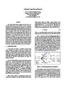
the activation-updating function (Bechtel & Abrahamsen, 1991; Rumelhart et al., 1986; Read & Montoya, 1999a). We present an autoassociative model with a recurrent architecture that uses a variant of delta-rule learning and that has an interactive activation- and competition-updating rule (these details will be explained shortly). In this recurrent network all nodes are completely connected to one another (with the exception that there are no self-connections), and there are weights or connections in both directions between each pair of nodes. A brief overview of these components follows. Architecture This refers to the way the network is structured in terms of connections. Some models comprise units that are only connected to a subset of the other units in the network, and some feed-forward networks, such as the pattern associator, use connections that send activation in only one direction, from an input set of units to an output set. We use an autoassociator in which the network is fully connected. Every unit is able to both receive information from and send information to every other unit in the network. However, the nodes do not have self-connections, that is, they are not connected to themselves. Further, every unit receives direct input from the environment and produces an output. (See Figure 1 for a small example.) Processing proceeds by presenting an input pattern of activation to all the units. The activation then flows among units. Because links go in both directions among all the nodes, the pattern of activation of the units in the network evolves over time and finally settles into a state that represents a solution to the constraints imposed by the links among the nodes and the inputs to them. One aim of the network is to learn how each unit’s activation has generally been associated with the others. Once the network has learned the associations among nodes, it can then use those associations to re-

Overview of Neural Network Models and our Model There are three important components of any neural network model: the architecture, the learning rule, and 150

Figure 1. Example recurrent network.


trieve information. For example, once the network has learned the association between a group name “college professor” and a characteristic of the group, “intelligent,” if the name of the group “college professor” is input to the network, it can “fill in” or retrieve the characteristic, “intelligent.” Localist versus distributed representation. Representation in connectionist models can either be localist or distributed. In a localist network, a concept, such as a group name or trait, is represented by a single node. By contrast, in a distributed network, a concept is represented by a pattern of activation across multiple nodes. For example, in our network, a group name is represented by a pattern of activation across 16 nodes and the attribute we use is also represented by 16 nodes. Among the advantages of a distributed representation are greater resistance to degradation of the representation and sensitivity to the degree of similarity between representations. This sensitivity to similarity between representations is central to this model. In distributed representations, memories are not located in any one location but rather are stored as a pattern of connection weights among a number of different nodes. Rumelhart et al. (1986) pointed out that distributed representations can give rise to powerful and sometimes unexpected emergent properties. For example, distributed representations enable retrieval of items from memory from partial descriptions, result in automatic generalization, and allow for the abstraction of prototypes. Exemplars versus prototypes. One obvious question about this model is whether memories are stored as exemplars or prototypes. McClelland and Rumelhart (1986) and Smith and DeCoster (1998a, 1998b) showed that this model can store both exemplars and prototypes, and that which one it stores is a function of the frequency distribution of the items. If the model receives a number of exemplars that are highly similar to one another, then they will be represented in terms of essentially the same pattern of weights, thereby creating a prototype; whereas if the exemplars are sufficiently different, the network will learn separate representations for each. In contrast, Park et al. (1991) argued that individuals learn abstractions or prototypes, and Linville et al. (1989) argued that individuals learn and store exemplars, although they do note that if an individual calculates a summary representation, as when making judgments such as variability, this summary representation can also be stored as an exemplar. The Learning Rule The learning rule for a network dictates how connections in a network are changed (strengthened or

weakened) in response to input during the learning process. The network learns the association among features, that is, the relations among activation values of nodes. In our simulations we use a variant of the delta rule (Widrow & Hoff, 1960), which is one of the most widely used learning rules. We first present the standard version of the rule, as it is easier to understand, and later present the variant that we used. The delta rule involves comparing the network’s output to the “correct” response (provided externally by a “teacher”) so that the network can correct its performance to better resemble the “correct” response. It is ∆wij = lr*e*aj where ∆wij is the change in the weight from node aj to node ai, lr is the learning rate, aj is the activation of the sending node and e is the difference between the target activation t and the actual activation of the receiving node ai (t – ai). Delta-rule learning is a form of error-correcting or predictive learning. The weight between the input and output node is modified as a function of the degree of error in the output node when the input node is activated. One important aspect of this rule is that learning decreases as the output error or the error of prediction decreases. This behavior of the delta rule contrasts with the well known Hebbian rule: ∆wij = lr*ai*aj The Hebbian rule does not have a term for error of prediction for the receiving node but, instead, has the activation of the receiving node. What the Hebbian rule does is essentially learn the degree of covariation between the activation of the two nodes. It is not sensitive to the error of prediction. If the two nodes are active at the same time, the weight between them is strengthened in proportion to the learning rate. And the degree of weight change is the same each time the two nodes are active together. Thus the weight change can increase without bounds. In contrast, with the delta rule, learning is asymptotic, decreasing as the error of prediction decreases. Reasons for delta-rule learning. There are several reasons why we use delta-rule learning. First, there is a large literature on both animal and human learning (e.g., Shanks, Holyoak, & Medin, 1996), which demonstrates that error-correcting learning rules, such as the Rescorla and Wagner (1972) rule or the formally identical delta rule (Widrow & Hoff, 1960), accurately describe a number of different aspects of learning that cannot be captured by rules that are not sensitive to errors in prediction. Second, networks with error-correcting learning rules, such as the delta rule or the gen151

READ AND URADA

eralization of the delta rule for multilayer networks, back propagation (Rumelhart et al., 1986), can learn things such as various aspects of language, which cannot be learned with Hebbian learning. Third, the model we use, with delta-rule learning, has already been successfully used to simulate various aspects of human memory (McClelland & Rumelhart, 1986), stereotype formation and change (Smith & DeCoster, 1998), and causal learning (Read & Montoya, 1999a). Finally, simple Hebbian learning is biologically completely implausible, as it predicts that weight strength could grow infinitely (although modified versions have been presented that do not have this problem). Clearly, biological constraints mandate some maximum weight strength. Error-correcting rules lead to asymptotic weight changes: Weight change diminishes as error of prediction decreases. Thus error-correcting rules have an upper limit for weight strength. One additional aspect of our learning rule is that weights decay with time. This allows us to capture the potential role of forgetting. Delta-rule learning with decay is defined as wij(t+1) = wij(t)*(1 - d) + ∆wij where

netI = (estr)*extinputI + (istr)*intinputI where extintputI is the external input to each node, and intinputI is the activation each node receives from other nodes in the network. Note that in calculating the net input, the internal and external activations are summed, whereas in applying the learning rule the internal and external activations are treated separately, as noted previously. Estr and istr are parameters that scale the external and internal inputs, respectively. In this simulation they were both set at .15, which is the value recommended by McClelland and Rumelhart (1986). Then the resulting activation of each node is calculated as follows: If (net i >0) a i (t + 1) = (1 - a i (t))*net i - decay*(a I (t)) Otherwise, a i (t + 1) = (a i (t) - - 1)*net i - decay*(a I (t))

where ai represents the activation of Unit a, neti represents the net input to Unit a from other sources, and decay is the rate of decay of activation for each unit (proportion from 0 to 1). This equation results in an S-shaped (or sigmoidal) activation function that keeps the maximum and minimum activation of a node between 1 and –1.

∆wij = lr*e*aj where wij represents the weight from unit j to unit i, t represents the previous time step, and t + 1 represents the current step; lr represents the learning rate, e or error represents the difference between the target (“correct”), and actual activation for unit ai, (t – ai), aj represents the activation of the input unit j, and d represents the decay rate, which is a proportion ranging from 0 to 1. This autoassociator uses a slight variant of delta-rule learning, as noted by McClelland and Rumelhart (1986). Here the external input to the network is treated as the target or teaching activation, and the internal input from all the other connected nodes is treated as the actual activation. Thus the network is trying to learn to have the internal activation accurately reproduce the external inputs. Activation Function This dictates how activation is propagated throughout a network. We used Rumelhart and McClelland’s interactive activation and competition function (McClelland & Rumelhart, 1981; Rumelhart & McClelland, 1982; Rumelhart et al., 1986). This function takes into account the current activation of each unit and the net input to the unit from other units and the external input, and then it uses these to compute a new activation strength for each unit as follows: First, the net input to a node is calculated as 152

Simulation In this simulation we examined the role of several aspects of the model in its ability to simulate the OHE. We orthogonally manipulated the learning rate, which affects the extent to which a weight is changed on each learning trial; the decay rate or forgetting rate, which is the proportion by which a weight decays on each learning trial; the ratio of in-group to out-group members; and the sample size—that is, how many total exemplars to which the model was exposed. In addition, we also manipulated attentional scaling, which is a constant by which the learning rate is multiplied when the network encounters an extreme exemplar (in the following simulations defined as high or low intelligence). This parameter is based on research showing increases in learning in humans when presented with extreme exemplars (Nisbett & Kunda, 1985; Rothbart, Fulero, Jensen, Howard, & Birrell, 1978; Walker & Jones, 1983). Linville et al. (1989) hypothesized that this increase in learning can play an important role in the OHE, and they set up their simulation so that learning was higher for instances falling at the upper and lower extreme of the distribution of abilities in their learning set. However, they fixed this parameter at a single value and did not manipulate it. Although they mention (p. 182) that they did try their simulations without this assumption and were still suc-


cessful, they provide no indication of what impact it had. Thus the extent to which it is responsible for their successful simulation of OHE cannot be determined. The rationale for why we expected these factors to influence the size of OHE will be clearer if one understands how information is represented in the model and how information is retrieved and used to estimate group variability. We first had our network learn about a number of individuals in two groups. For current purposes we will refer to the two groups simply as the in-group and the out-group. Each individual in the two groups had one of 5 levels of a characteristic, which we will refer to as intelligence, to be concrete. The levels of intelligence had a quasi-normal distribution, such that for every 5 individuals with average intelligence, there were 3 with either below-average or above-average intelligence, and 1 with either high or low intelligence (1 3 5 3 1). Measurement of Variability In our recurrent model, variability is not directly stored, as is also true for the models of Fiedler et al. (1999), Kraus et al. (1993), and Linville et al. (1989). Rather, variability is computed by querying the network as to how much it knows or remembers about each level on the continuum and then computing variability from that response. We measured group variability by analogy to the technique that Linville et al. (1989) used. Linville et al. (1989) probed their exemplar-based memory with a question about each type of individual the model had seen and then measured the strength of response to the question. In their model the response can be thought of as due to a resonance or tuning-fork-type process. A probe is entered into the memory, and exemplars in the memory that are similar to the probe send a response. The more different exemplars resonate to the probe, the stronger the response. Thus, in their model the response to the probe is a function of how many similar exemplars are in the memory, where this is a function of such things as the number of exemplars seen, the probability that an item is learned, and the probability that a learned item is subsequently forgotten. For example, if one wanted to characterize the distribution of safety records of New York cab drivers, one would enter several different probes into the network ranging from “New York cab drivers are very safe” to “New York cab drivers are very dangerous” and “listen” for the response from the network. The relative strength of response to those probes would allow you to judge how variable New York cab drivers are on safety. If on a range from 7 (very dangerous) to 1 (very safe), by far the strongest response was from very dangerous, and there were weak responses for the other levels, then one could calculate that there is little variability in dangerousness. However, if there were a

fairly similar response at all levels, then variability would be quite high. An analogous strategy was used for our recurrent neural network. Once the network has learned, one can test the strength of response of a recurrent network to a particular pattern by presenting that pattern and allowing the network to iterate for a number of cycles until it settles. The strength of activation of the resulting pattern is a function of how well the network has learned the pattern corresponding to the probe, which is a function of such things as frequency of occurrence and learning rate. Thus we can measure the strength of response at each level of the attribute by using a probe consisting of a pattern corresponding to the group name and the probed level of the characteristic, and then using these responses to calculate the variability of the group on that characteristic. The strength of the response to a probe was calculated by using the normalized dot product between the probe vector and the retrieved vector. McClelland and Rumelhart (1986) recommended this as a measure of the degree to which an output pattern of activation captures the original input pattern. The formula used was αp = (1/n)Σaiepi where p indexes the pattern presented, i indexes the units in the network, a indexes the response vector, epi indexes the external input to unit i from pattern p, and n is the number of elements in the pattern. When we use the strength of response from each level in a quasi-normal distribution to calculate variability, then the relative strength of response of extremes versus middle values plays a major role in the degree of variability. One implication of this is that the relative strength of learning of extreme values compared to the central value is important. The greater the learning of the extremes compared to the central value, the stronger the relative response of the extremes and, thus, the higher the variability. Conversely, if the central value is learned extremely well, but the extremes poorly, then variability will be low. Thus any factor that increases the relative learning of the extreme values compared to the middle values should increase the variability estimate.

Parameters Manipulated A number of factors may potentially affect the relative strength of learning of extremes compared to the middle values in the autoassociative model. In this simulation we examine five factors: (a) the relative frequency of exposure to members of the in-group versus the out-group, (b) the overall frequency of exposure to exemplars of the entire population, (c) the extent to which extreme values are better learned than mean val153

READ AND URADA

ues, (d) the learning rate or degree of learning from each instance, and (e) the decay rate for weights. One important factor in the relative learning for mean versus extreme values is the frequency with which exemplars are encountered. This follows from the asymptotic nature of delta-rule learning. Because learning is a function of the difference between the target and the output value, the closer the output is to the target, the smaller the weight change. Thus the better the network learns the relation between nodes, the smaller the change on subsequent encounters with a stimulus. More exemplars result in better learning, but the impact of each exemplar decreases asymptotically with more exemplars. Assume that the distribution of instances is quasi-normal. In such a distribution far more exemplars of the middle value are encountered than of the extremes. Thus asymptotic learning will be reached sooner for middle values than for extreme values. However, if a large enough number of exemplars are encountered, then eventually asymptotic learning will occur for both the middle and the extremes. This suggests that as long as learning has not yet reached asymptote, then fewer exemplars will result in lower variability (i.e., greater perceived homogeneity). Thus if one is comparing two samples of different sizes, the larger sample will be more likely to be closer to asymptotic values than will the smaller. As a result, the larger sample should have higher variability. This conclusion is consistent with the prediction and demonstration that the OHE is most likely when there is greater exposure to members of the in-group than the out-group (Ostrom & Sedikides, 1992). (However, the fact that the OHE is occasionally found for 1:1 ratios of in-group to out-group suggests that other factors may also play a role in the OHE.) In-group–out-group ratio. In our simulation, we manipulated the relative size of the in-group and the out-group to attempt to demonstrate that in this model the OHE is at least partially a function of lesser familiarity with the out-group relative to the in-group. Any adequate model of the OHE should be sensitive to such differences in relative familiarity. The ratios used were 5:2 and 10:2. We did not use an equal ratio (i.e., 1:1) because in this model there would be no difference in variability judgments for two groups with equal numbers of exemplars. Further, none of the other manipulations would have any impact on differential variability when the two groups are equally frequent. Population size. In addition to manipulating the in-group–out-group ratio, we also orthogonally manipulated the absolute number of exemplars encountered for both groups. That is, for each of the two ratios, we had three different sample sizes: the base size, double the base size, and 4 times the base size. Given the pre154

ceding analysis of asymptotic learning, increasing the sample size should reduce the differences in variability between the two groups. Learning of extreme values. A third factor that should affect relative learning of extremes compared to middle values is greater attention to extreme cases. Linville et al. (1989), based on earlier work by Rothbart et al. (1978), argued that people are more likely to remember extreme exemplars from a population. They implemented this greater learning of extremes in their model. However, because they never manipulated the degree of learning of extremes in the published account of their model, it is impossible to tell what role this factor played in the success of their simulation. In this simulation we explicitly manipulate this factor at 3 levels. Because preliminary simulations showed that a scaling of 3 times the base learning level led to strange results, we used the square root of these integers as the scaling factor: 1, √2, √3. Learning rate. A fourth factor that should affect relative learning is the learning rate. The learning rate in delta-rule learning is the proportion of the error signal by which the relevant weight is changed. For example, if the error signal (target – actual) is .33, and the learning rate is .01, then the relevant weight will be incremented by .01 × .33 = .0033. With a higher learning rate, weight changes will occur in bigger steps and learning will, as a result, typically occur more quickly. (However, if the learning rate is too large, the network may essentially keep jumping around and never find the best solution. Thus in neural networks it is important not to make weight changes too large.) One implication of a larger learning rate is that it should reduce the difference in learning between middle and extreme values. One way to think of this is that with larger learning rates (within some limit) extreme cases will reach maximal learning with fewer instances. Weight decay rate. We also wondered whether the weight decay rate would influence the OHE. Intuitively, decay in weight strength might have a greater impact on the extremes, where learning is relatively poor, than on the middle values. This would reduce variability. However, it may also be that differences in decay will have the opposite impact. In this model, decay is implemented as a proportional decrease in the current weight strength. Thus a proportional decrease in a large weight will lead to a greater change than the same proportional change in a small weight. For example, a 10% decay in a .5 weight is .05, whereas a 10% change in a .10 weight is .01. Thus there will be greater unlearning for large weights than for small weights. This should increase variability by decreasing the relative strength of middle values compared to extreme values.


Method Materials All of the simulations were run using MATLAB software version 5.1.0.420 (MathWorks, Inc., Natick, MA, 1997) with MathWorks’ supplemental Neural Network Toolbox, Version 3.0 (Demuth & Beale, 1994). We used a 32-unit, fully connected network. Sixteen of the units represented the group name and 16 represented the level of the characteristic we were using. Target vectors. For stimuli, we created a number of 32-element target vectors, each of which represented a single person. Each element in the vector had a value of either –1 or +1. The first 16 elements of the vector represented group membership. The pattern was random, and we refer to these group memberships as in-group and out-group. The in-group and out-group patterns we used were orthogonal, having a zero correlation with each other. The second 16 elements in each vector represented a level of a trait. Although any trait could be substituted, for illustration these elements represent intelligence. To represent 5 levels of intelligence, five 16-element patterns were created. These patterns were nonorthogonal to one another and were created in such a way that the degree of overlap or similarity among vectors represented the relative rank ordering of the attributes. We used a 16-element vector to code a 5-level attribute as follows: Start with a vector that codes the lowest level, say well below average intelligence. To code the next highest level, below-average intelligence, randomly reverse the values of 4 elements, from 1 to –1 or –1 to 1. Then to code the next level, average intelligence, randomly reverse 4 more elements (8 out of 16 reversed). Then to code above average, reverse 4 more, and to code well above average, reverse the remaining 4 elements. With this scheme, the degree of overlap between vectors captures how distant they are from each other. One way to see this is to look at the normalized dot product between vectors, which is akin to the correlation. The normalized dot products of the lowest value with the other four, in order, are .5, 0, –.5, and –1. The normalized dot products of Level 2 with 3, 4, and 5 are .5, 0, and –.5, respectively. And the normalized dot product of the middle value is .5 with the two adjacent values and 0 with the two extremes. Thus the pattern of relations among these vectors codes their relative rankings and, therefore, roughly captures the level of the attribute. In contrast, if purely orthogonal codings had been used, the correspondence of a vector with the level of an attribute would be totally arbitrary, and the simulation would not be sensitive to the similarity of adjacent attributes. Such overlapping vectors have

been used in a number of contexts to code different levels of an attribute. We then constructed vectors that represented 10 different types of people varying on group membership (in-group, out-group) and intelligence (very low, low, average, high, and very high). All of the different combinations and the patterns associated with each are shown in Table 1. Population matrices. Having constructed vectors representing various “people,” we then put these together to create matrices representing populations of in-group and out-group members of varying intelligence levels. We first created two population matrices, each containing a different ratio of in-group to out-group members (5:2 and 10:2). We then varied the population size for each ratio, at one of 3 levels: the initial population size, double the initial size, and quadruple the initial size. The different combinations that were created and used are shown in Table 2. The distribution of intelligence levels among in-group and out-group was identical. Within each group we varied the number of people at each intelligence level to conform to a 1:3:5:3:1 quasi-normal ratio. That is, for each group only a small proportion of people were of either very low or very high intelligence, but a relatively large proportion were of average intelligence. Procedures To assess the impact of each parameter, we varied the relative proportions of in-group to out-group, the overall population size, scaling of attention to extreme values (attentional scaling), the weight decay rate, and the learning rate. Our design was a 2 (ratio of in-group to out-group: 5:2, 10:2) × 3 (population size: base size, double, and quadruple size) × 3 (attentional scaling: 1, Table 1. Input Vectors Used for the Simulations Group Name

Levels of Intelligence

In-group

Out-group

1

2

3

4

5

+1 +1 –1 –1 –1 –1 +1 +1 +1 +1 –1 –1 –1 –1 +1 +1

+1 +1 +1 +1 –1 –1 –1 –1 –1 –1 –1 –1 +1 +1 +1 +1

–1 –1 +1 +1 –1 –1 +1 +1 –1 –1 +1 +1 –1 –1 +1 +1

–1 –1 +1 –1 –1 –1 +1 –1 –1 –1 +1 –1 –1 –1 +1 –1

–1 –1 –1 –1 –1 –1 –1 –1 –1 –1 –1 –1 –1 –1 –1 –1

+1 –1 –1 –1 +1 –1 –1 –1 +1 –1 –1 –1 +1 –1 –1 –1

+1 +1 –1 –1 +1 +1 –1 –1 +1 +1 –1 –1 +1 +1 –1 –1

155

156

Quadruple sample

Double sample

Initial sample

Sample Size 5:2 10:2 5:2 10:2 5:2 10:2

In-group— Out-group Ratio

Table 2. Population Matrices Used

65 130 130 260 260 520

Total Number of In-group Members 5, 15, 25, 15, 5 10, 30, 50, 30, 10 10, 30, 50, 30, 10 20, 60, 100, 60, 20 20, 60, 100, 60, 20 40, 120, 200, 120, 40

Number of In-group Members at Intelligence Levels 1, 2, 3, 4, 5 26 26 52 52 104 104

Total Number of Out-group Members

2, 6, 10, 6, 2 2, 6, 10, 6, 2 4, 12, 20, 12, 4 4, 12, 20, 12, 4 8, 24, 40, 24, 8 8, 24, 40, 24, 8

Number of Out-group Members at Intelligence Levels 1, 2, 3, 4, 5


√2, √3) × 5 (decay rate: .01, .02, .03, .04, .05) × 5 (learning rate: .002, .004, .006, .008, .01) analysis of variance (ANOVA). The learning rate varied from .002 to .01 because, in earlier versions of the simulation, we had varied learning rate from .01 to .05, and we found that at learning rates much above .01, there were a large number of cases with negative variances. Negative variance estimates are possible in this situation because the formula we used to estimate variances relies on the dot product between the input and the output vector to estimate the proportion of a response that comes from different levels of the attribute. This dot product, and the resulting proportion, can be negative in some cases. Consistent with our problems on the earlier simulations, McClelland and Rumelhart (1986) argued, on the basis of considerable experience, that learning rates with this type of model should not exceed 1/(number of nodes), which in this network is 1/32 = .031. Learning rates that are too high lead to poorly behaved networks. Thus we decided to look at learning rates of .01 or less. As explained in the following section, 50 separate simulations were run for each of the 450 cells or combinations of these parameters. Each simulation proceeded through three discrete phases. During the first phase, the network was exposed to the population stimuli and learned. During the second phase, the network was tested for recognition of the patterns it had learned during the previous phase. Finally, in the third phase the retrieved patterns were used to compute the variability of each group and, thus, their relative homogeneity. Learning phase. The population matrices were used as input for the network. During each simulation the network was exposed to each target “person” or vector from the population matrix, one at a time. Because the order of target presentation can impact the storage of target information (targets presented later tend to be retrieved more easily), we randomized the order in which the targets from the population matrix were presented during learning. This was achieved by randomly sampling from the population matrix without reusing any targets until all of the targets had been used. A different random order was used for each of the 50 simulations in a cell. Each target was input by fixing the activation of the nodes in the network in a pattern that corresponded to the target pattern and then allowing the activation to spread and settle over 50 iterations. Once the activation stopped spreading, the strength of the connections between units was changed using the delta-learning rule. The next vector or “person” was then presented to the network, and the process was repeated until all of the vectors in the population matrix had been presented. Psychologically, this process

is the equivalent of meeting (or at least observing) many different people in succession. Recognition phase. After completion of the learning phase, the network was then tested for how well it recognized each of the 10 individuals. To do this, the network was sequentially given one vector of each target type, by clamping the input activations on the units, and the response of the network to each was tested (e.g., in-group intelligence Level 1, out-group intelligence Level 1, in-group intelligence Level 2, out-group intelligence Level 2, and so on.). Psychologically, this might be considered the equivalent of being asked, “Can you remember meeting anyone like this?” The network was allowed to settle using the interactive activation and competition function. To ensure complete settling of the network, 50 iterations were allowed. No learning took place during this phase. Calculation of variability. To determine the strength of recognition, normalized dot products between each of the original target vectors and the retrieved vector corresponding to it were computed. McClelland and Rumelhart (1986) recommended this as a measure of the degree to which an output pattern of activation captures the original input pattern. The formula used was αp = (1/n)Σaiepi where αp is the dot product for the two n-element vectors (here n is 32), p indexes the pattern presented, i indexes the units in the network, ai indexes the elements of the response vector or retrieved vector, epi indexes the external input to Unit i from Pattern p, which here is the target or test vector, and n is the number of elements in the pattern. In calculating a normalized dot product, the corresponding pairs of elements in two vectors are multiplied, and then these products of pairs are summed, and the sum is divided by the number of elements in the vector. That is, the first element in one vector is multiplied by the first element in the other, the second element in the first vector is multiplied by the second element in the other, and so forth. Then the products are summed and divided by the number of pairs. The result is conceptually similar to calculating the covariances between the two vectors, being sensitive both to similarity in the form of the two patterns and the strength of their individual elements. For each simulation, the dot products for each target vector were recorded, and then using Linville et al.’s (1989) procedure, the variability was calculated for the in-group and the out-group as follows. First, the proportion of total pattern activation (dot products) contributed by each level of intelligence was computed. 157

READ AND URADA

For example, for in-group of intelligence Level 5, the computation was PI5 = dI5/dItotal where PI5 was the proportion of the total pattern activation contributed by in-group members with an intelligence level of 5, dI5 was the dot product for in-group intelligence Level 5, and dItotal was the sum of the dot products for in-group members of all intelligence levels. Then the variability of the perceived distribution was computed using an adapted version of the formula used by Linville et al. (1989, p. 167) to compute perceived variability of the Group G (in-group or out-group): VarGi = Σi= 1,mPGi(Xi-M)2 where m is the number of levels of the attribute, PGi is the proportion of total activation of Group G at Level i, Xi is the intelligence scale value (1–5) for vectori and M denotes the mean of the perceived distribution (M = Σi=1,mPIiXi). Finally, the difference between the in-group variance and the out-group variance was computed to give an overall OHE score. Positive values on this measure indicate greater variability for the in-group compared to the out-group and, therefore, greater homogeneity for the out-group. To control for results arising from the order in which exemplars were learned, the entire process up to this point, from randomization of target order, to testing, to calculation of variance and the size of the OHE, was repeated 50 times for each combination of parameters. Thus there were 50 simulations for each of 450 combinations of parameters, giving us 22,500 data points.

Results To determine whether each parameter influenced out-group homogeneity, the results of the simulation were subjected to ANOVA. As explained previously, the design of the simulation was a 2 (ratio of in-group to out-group: 5:2, 10:2) × 3 (population size: base size, double, and quadruple size) × 3 (attentional scaling: 1, √2, √3) × 5 (decay rate: .01, .02, .03, .04, .05) × 5 (learning rate: .002, .004, .006, .008, .01). Fifty separate simulations, with different orders of random sampling of the population, were run for each combination of parameters in the design. The output of each simulation was treated as one subject. This approach to simulation has previously been used by Fiedler et al. (1999), Hintzman (1988), and Linville et al. (1989). We performed separate ANOVAs for the OHE (in-group variance—out-group variance) and for the variance esti158

mates for the in-group and out-group separately, so that we could determine the extent to which changes in the OHE were due to the in-group versus the out-group. In the analyses we had to exclude 438 out of 22,500 cases for negative variances. There were no negative variances in the lowest scaling condition, 18 in the Level 2 scaling, and the remaining 420 were in the Level 3 scaling condition. Further, within the scaling conditions, the negative variances increased as the learning rate increased. This suggests that setting learning and particularly attentional scaling at too high a level can result in poorly behaved networks. In performing these analyses on Statistical Package for the Social Science (SPSS; version 10 for the MacIntosh), we ran into a serious memory problem that made it impossible to perform the overall ANOVAs on a computer with 256MB of memory. The full design has 450 cells with approximately 22,000 subjects. To reduce the size of the analysis, instead of analyzing all 5 levels of both learning and decay rate, we analyzed the 1st, 3rd, and 5th level of each. Preliminary viewing of the means for all 5 levels suggested that this would allow us to capture the impact of these two factors, without any serious distortions of the results. This reduced this aspect of the design from a 5 × 5 = 25 to a 3 × 3 = 9, and, thus, the overall analysis was reduced from 450 cells to 162. With this reduction, we were able to perform the analyses. The output of the resulting ANOVAs is reported in the following sections. Because the sample size is quite large, even with this reduced analysis, and the standard errors are small, even fairly small mean differences were sometimes significant. Thus to reduce the reporting of a number of statistically significant, but relatively trivial results, only significant results with an η2 of over 2% are reported. Further, to provide an idea of the size of various results, we report η2 for all reported results. Main Effects OHE. First, there was a significant overall OHE effect, with the overall mean being significantly different from 0, M = .828, F(1, 7802) = 1,317,586.47, p < .001. The individual variance components were also highly significant, in-group: M = 1.608, F(1, 7802) = 118,220,718, p < .001 and out-group: M = .780, F(1, 7802) = 1,165,010.37, p < .001. In-group–out-group ratio. As expected, there was a main effect of the ratio of in-group to out-group members, F(1, 7802) = 6,767.36, p < .001, η2 = .464, with the OHE increasing as the ratio of in-group to out-group size rose (see bottom, Table 3). This seemed to be largely due to a decrease in out-group variance with increasing ratios, F(1, 7802) = 5,990.53, p < .001, η2 = .434. The increase in in-group variance, although


Table 3. Ingroup/Outgroup Ratio by Attentional Scaling

Table 5. Learning Rate by Population Size

Ingroup/Outgroup Ratio Attentional Scaling

Learning Rate

5:2

10:2

Average

OHE In-Group Out-Group

.711 1.588 .877

.856 1.603 .747

.784 1.596 .812


.776 1.604 .828

.890 1.611 .720

.833 1.607 .774

OHE In-Group Out-Group Average OHE In-Group Out-Group

.819 1.621 .802

.917 1.620 .704

.868 1.621 .753

.769 1.604 .835

.888 1.611 .724

.828 1.608 .780

1

2

3

Population Size Base OHE In-Group Out-Group Double OHE In-Group Out-Group Quadruple OHE In-Group Out-Group Average OHE In-Group Out-Group

.002

.006

.010

.717 1.626 .909

.873 1.61 .736

.899 1.608 .709

.773 1.613 .839

.859 1.603 .745

.867 1.605 .737

.793 1.604 .811

.828 1.599 .772

.846 1.602 .757

.761 1.614 .853

.853 1.604 .751

.871 1.605 .735

quite small, was still significant, F(1, 7802) = 548.45, p < .001, η2 = .066.

variance with increasing decay rate for the in-group, F(4, 7802) = 117.86, p < .001, η2 = .029.

Attentional scaling. The size of the OHE increased with increased attentional scaling, F(2, 7802) = 1,138.44, p < .001, η2 = .226 (see far-right column, Table 3). This resulted from a significant increase in in-group variance with increased scaling, F(2, 7802) = 2,361.94, p < .001, η2 = .377, and a significant decrease in out-group variance with attentional scaling, F(2, 7802) = 571.30, p < .001, η2 = .128.

Learning rate. The size of the OHE increased as the learning rate increased, F(2, 7802) = 2,230.27, p < .001, η2 = .364 (see bottom, Table 5). This was due largely to a drop in the out-group variance as the learning rate increased F(2, 7802) = 2661.46, p < .001, η2 = .406, with a smaller drop in the in-group variance, F(2, 7802) = 484.50, p < .001, η2 = .110.1

Decay rate. The size of the OHE decreased as the decay rate increased, F(4, 7802) = 2295.67, p < .001, l2 = .370 (see bottom, Table 4). This was a result of a significant increase in variance with increasing decay rate for the out-group, F(4, 7802) = 2,085.33, p = .001, η2 = .348, and a small, but significant, decrease in

Interactions

Table 4. Decay Rate by Attentional scaling Decay Rate Attentional Scaling

.01

.03

.05


.859 1.596 .736

.765 1.596 .831

.727 1.595 .868


.905 1.607 .702

.817 1.608 .791

.777 1.607 .830

OHE In-Group Out-Group Average OHE In-Group Out-Group

.916 1.630 .715

.866 1.617 .751

.822 1.615 .793

.893 1.611 .718

.816 1.607 .791

.775 1.606 .830

1

In-group–out-group ratio by attentional scaling. The increase in OHE with larger in-group–out-group ratios diminished at higher levels of attentional scaling, F(2, 7802) = 91.74, p < .001, η2 = .023 (see Table 6). This was due both to the out-group variance component, F(2, 7802) = 41.64, p < .001, η2 = .011, where the decrease in out-group variance with higher in-group–out-group ratios diminished at higher levels of attentional scaling, and to the in-group variance component, where the increase in in-group variance with higher ratios decreased at higher scaling levels, F(2, 7802) = 240.93, p < .001, η2 = .058.

2

3

In-group–out-group ratio by learning rate. The increase in OHE with larger in-group–out-group ratios 1The results for population size, although somewhat interesting, did not reach the criterion of 2% of the variance. The size of the OHE decreased slightly as the population increased, F(2, 7802) = 20.70, p < .001, η2 = .005 (see bottom, Table 6). This was a result of a decrease in in-group variance as the population size increased, F(2, 7802) = 598.94, p < .001, η2 = .133, and a smaller decrease in out-group variance as the population size increased, F(2, 7802) = 20.32, p < .001, η2 = .005.

159

READ AND URADA

Table 6. Population Size by Attentional scaling

Table 8. In-Group/Out-Group Ratio by Decay Rate

Population Size Attentional Scaling

Decay Rate

Base

Double

Quad


.776 1.596 .820

.791 1.595 .804

.784 1.595 .812


.833 1.614 .782

.841 1.606 .765

.827 1.601 .775

OHE In-Group Out-Group Total OHE In-Group Out-Group

.880 1.633 .753

.868 1.620 .752

.856 1.609 .753

.830 1.615 .785

.833 1.607 .774

.822 1.602 .780

.01

1

2


.03

5:2

10:2

5:2

10:2

5:2

10:2

.853 1.610 .757

.934 1.612 .678

.752 1.603 .851

.880 1.611 .731

.701 1.600 .899

.849 1.611 .762

Table 9. In-Group/Out-Group Ratio by Population Size

3

decreased with higher learning rates, OHE F(2, 7802) = 1217.37, p < .001, η2 = .238 (see Table 7). This was largely due to the out-group variance component, where, as the learning rate increased, the variance dropped more sharply for the 5:2 ratio, then for the 10:2 ratio condition, F(2, 7802) = 1134.28, p < .001, η2 = .225. In-group–out-group ratio by decay rate. The impact of in-group–out-group ratio was greater for higher decay rates (see Table 8), F(2, 7802) = 192.58, p < .001, η2 = .047. This effect was largely due to the out-group, where the decrease in variance with larger in-group–out-group ratios became larger as the decay rate increased, F(2, 7802) = 138.52, p < .001, η2 = .034. There was also a tendency for the in-group variance to increase more strongly with higher ratios as the decay rate increased, F(2, 7802) = 105.01, p < .001, η2 = .026. In-group–out-group ratio by population size. The size of the increase in OHE with larger in-group–out-group ratio decreased as the population size increased, F(2, 7802) = 226.32, p < .001, η2 = .055 (see Table 9). This was largely due to the out-group variance component, where the drop in variance from 5:2 to 10:2 ratios was less sharp for larger population Table 7. In-Group/Out-Group Ratio by Learning Rate Learning Rate .002


160

.006

.010

5:2

10:2

5:2

10:2

5:2

10:2

.652 1.609 .957

.870 1.619 .749

.811 1.601 .790

.895 1.608 .712

.844 1.603 .760

.898 1.607 .709

.05

Population Size Single


Double

Quadruple

5:2

10:2

5:2

10:2

5:2

10:2

.751 1.611 .861

.908 1.618 .709

.775 1.604 .828

.891 1.611 .719

.781 1.599 .818

.863 1.606 .742

Table 10. Learning Rate by Attentional scaling Learning Rate

Attentional Scaling 1 OHE In-Group Out-Group Attentional Scaling 2 OHE In-Group Out-Group Attentional Scaling 3 OHE In-Group Out-Group

.002

.006

.010

.714 1.595 .881

.806 1.595 .789

.831 1.596 .765

.764 1.616 .852

.857 1.604 .747

.879 1.602 .723

.805 1.632 .826

.896 1.614 .717

.902 1.617 .715

sizes, F(2, 7802) = 228.34, p < .001, η2 = .055. Consistent with our earlier predictions, larger population sizes reduced the impact of larger in-group–out-group ratios on out-group variances. Population size by learning rate. The size of the increase in the OHE with higher learning rates decreased as the population size increased, F(4, 7802) = 293.22, p < .001, η2 = .131 (see Table 5). This was largely due to the out-group variances, where the decrease in out-group variance with greater learning was smaller with larger populations, F(4, 7802) = 361.34, p < .001, η2 = .156. The in-group variances showed a pattern similar to but weaker than the out-group variances F(4, 7802) = 90.58, p < .001, η2 = .044.2 2Three interactions, although somewhat interesting, did not reach the criterion of 2%. Attentional scaling by decay rate. Although the size of the OHE decreased with higher decay rates, the amount of decrease with greater decay diminished with higher attentional scaling, F(4, 7802)


Attentional scaling by learning rate by decay rate. Although this three-way interaction was significant for all three components (OHE F(8, 7802) = 30.78, p < .001, η2 = .031; in-group F(8, 7802) = 47.05, p < .001, η2 = .046; out-group F(8, 7802) = 47.80, p < .001, η2 = .047; see Table 11), the effects do not seem to be particularly meaningful.

Discussion As predicted, the degree of differential familiarity with the out-group versus the in-group played a central role in the occurrence of the OHE. The greater the familiarity with the in-group compared to the out-group, the larger the OHE. This is supported both by the difference between the 5:2 and the 10:2 ratios, and the significant difference of the OHE from 0 at the 5:2 ratio. The result was largely due to a substantial decrease in out-group variance with increasing ratios. As the number of in-group members relative to out-group members increased (increasing in-group–out-group ratio), the out-group variance decreased. The differences in results between in-group and out-group variances seem quite reasonable. In-group variance estimates were probably near asymptote and, thus, were relatively unaffected by the manipulations. In contrast, out-group variance estimates were affected by the decreasing proportion of out-group members in the population. This is consistent with Linville et al.’s (1989) findings and simulation. It is also consistent with Linville and Fischer’s (1993) review of the implications of four categorization models for the OHE, in which they noted that in all of these models, differential familiarity with the in-group relative to the out-group would be = 36.40, p < .001, η2 = .018 (see Table 4). For the out-group, the amount of increase in out-group variance with greater decay rates diminished at higher levels of attentional scaling, F(4, 7802) = 67.30, p < .001, η2 = .033. In contrast, for the in-group variance, the impact of decay rate was slightly higher for higher scaling, F(4, 7802) = 118.32, p < .001, η2 = .057. Attentional scaling by learning rate. Although this interaction was significant for both the OHE, F(4, 7802) = 8.29, p < .001, η2 = .004 and the in-group variances, F(4, 7802) = 10.91, p < .001, η2 = .006 (see Table 10), neither interaction accounted for much variance. Only the out-group variance component accounted for much variance, F(4, 7802) = 150.59, p < .001, η2 = .072. Essentially, the decrease in out-group variance with increased learning rate, decreased with greater attentional scaling. This would make sense given that increased learning rate seems to have had a greater impact on relative learning of central values, whereas attentional scaling would lead to greater learning of extreme values. Attentional scaling by population size. The interaction for OHE was small, although significant, F(4, 7802) = 15.34, p < .001, η2 = .008 (see Table 6), as was also true for the out-group component, F(4, 7802) = 3.80, p = .01, η2 = .002. However, for in-group variances, the extent of the positive impact of scaling decreased with increasing population size, F(4, 7802) = 157.54, p < .001, η2 = .075.

necessary to get the OHE, and it is consistent with Fiedler et al.’s (1999) analysis. The impact of differential familiarity is also consistent with Mullen and Hu’s (1989) meta-analysis of the OHE. For attentional scaling, the size of the OHE increased with increased attentional scaling. This resulted from a small, but significant increase in in-group variance with increased scaling and a significant decrease in out-group variance with attentional scaling. The increase in in-group variance with increased scaling makes sense, given that it should lead to greater learning of extreme values. However, the decrease in out-group variance with increased scaling is a little puzzling. Although the influence of attentional scaling is consistent with Linville et al.’s (1989) emphasis on the role of increased learning of extreme values, it is important Table 11. Attentional Scaling by Learning Rate by Decay Rate Decay Rate

Attentional Scaling 1 Learning Rate .002 OHE In-Group Out-Group Learning Rate .006 OHE In-Group Out-Group Learning rate .010 OHE In-Group Out-Group Attentional Scaling 2 Learning Rate .002 OHE In-Group Out-Group Learning Rate .006 OHE In-Group Out-Group Learning rate .010 OHE In-Group Out-Group Attentional Scaling 3 Learning Rate .002 OHE In-Group Out-Group Learning Rate .006 OHE In-Group Out-Group Learning rate .010 OHE In-Group Out-Group

.01

.03

.05

.777 1.596 .819

.695 1.595 .900

.669 1.594 .925

.886 1.596 .710

.784 1.596 .812

.750 1.595 .845

.915 1.595 .680

.817 1.598 .781

.762 1.596 .835

.834 1.616 .782

.742 1.616 .875

.716 1.616 .900

.934 1.602 .669

.842 1.605 .763

.795 1.604 .808

.948 1.603 .654

.868 1.602 .734

.821 1.602 .781

.883 1.633 .750

.785 1.632 .846

.748 1.630 .882

.955 1.620 .665

.890 1.611 .721

.844 1.610 .766

.909 1.638 .729

.922 1.608 .686

.874 1.605 .730

161

READ AND URADA

to note that the OHE was quite strong even without such increased learning of extremes. Thus, at least in this model (and also in Fiedler et al.’s 1999 model), increased learning of extreme values is not necessary for the OHE. The OHE decreased as the decay rate increased. This was largely the result of a significant increase in variance with increasing decay rate for the out-group. The increase in out-group variance with greater weight decay suggests that the weight strengths representing central attributes were more strongly affected than for extremes, which is consistent with weight decay being implemented as a proportional decrease in weight strength. Reduced strength of central values compared to extremes should lead to higher variances because a higher proportion of the activation will come from extremes. Interestingly, the OHE increased as the learning rate increased, largely because of a drop in the out-group variances with an increasing learning rate. The decrease in variances with a higher learning rate suggests that as the learning rate increased, the relative learning of central values compared to extreme values increased. Because the calculation of variances is based on the proportion of activation from each of the attribute levels, if a larger proportion of the total activation comes from the central value, then a smaller proportion would come from the extreme values and as a result the variance estimates would decrease. Increased population size led to a decreased OHE, largely because of a decrease in in-group variance. Although the decrease in the OHE with larger populations was predicted, the finding that it was due to a decrease in in-group variance with larger population was somewhat unexpected. We had been expecting it to be due to an increase in the out-group variance. One possible reason is that larger sample sizes led to increased learning of central values compared to extremes, particularly for the in-group. In addition to the various main effects of the manipulated parameters, the impact of in-group–out-group ratio was moderated by each of the other four parameters: attentional scaling, population size, decay rate, and learning rate. First, as expected, the size of the increase in OHE with larger in-group–out-group ratio decreased as the population size increased. This suggests that the OHE should be smaller in larger populations. Second, the increase in the OHE with larger in-group–out-group ratios diminished at higher levels of attentional scaling. Third, the increase in OHE with larger in-group–out-group ratios also decreased as the learning rate increased, suggesting that factors that increase learning might reduce the OHE. Evidently, each of these three factors, population size, learning rate, and attentional scaling reduces the difference in variance estimates between the in-group and the out-group. Finally, the 162

impact of in-group–out-group ratio was greater as the decay rate increased. It is also worth noting that, in general, the various manipulations had a greater impact on the out-group variances than on the in-group variances. Presumably this occurred because the in-group variances were already close to their asymptotic values and could not be moved around as much. Interestingly, there may have been some degree of competition in learning relations to attribute values for the in-group versus the out-group. In several cases, the same parameter had opposite effects on in-group and out-group variances. For example, in-group variance increased with increased attentional scaling, whereas out-group variance decreased with increased attentional scaling Centrality of Error-Correcting Learning to This Simulation Central to the ability of this model to capture the OHE is the error-correcting nature of delta-rule learning. In delta-rule learning the degree of learning or weight change is a function of the size of the discrepancy between the target value (t) and the actual value (a), the error, or alternatively, of the accuracy of the prediction. ∆wij = lr*(t-aI)*aj As can be seen in this equation, as the discrepancy or error decreases the extent of weight change or learning also decreases. So learning or weight change, with error-correcting learning, is asymptotic: It starts out relatively large when the discrepancy or error is large but decreases in size as the discrepancy decreases. The role of delta-rule learning in the OHE can be better seen with a concrete example. Here we consider a normal or quasi-normal distribution. In this model we use the strength of response from each point in a distribution to calculate variability. Therefore, with a quasi-normal distribution, the relative strength of response of extremes versus middle values plays a major role in the degree of variability. And because the strength of response depends on the degree of learning, the relative degree of learning of extreme values compared to central values is important. The greater the learning of the extremes compared to the central value, the stronger the relative response of the extremes and, thus, the higher the variability. Conversely, if the central value is learned extremely well, but the extremes are learned poorly, then variability will be low. Any factor that increases the relative learning of the extreme values compared to the middle values will increase the variability estimate. Because of the asymptotic nature of delta-rule learning, one important factor in the relative learning for mean versus extreme values in a quasi-normal dis-


tribution is the size of the sample that is encountered. In a quasi-normal distribution, far more exemplars of the middle value are encountered than of the extremes. Thus asymptotic learning will be reached sooner for middle values than for extreme values. However, if a large enough number of exemplars is encountered, then eventually asymptotic learning will occur for both the middle and the extremes. This suggests that if one is comparing learning from two samples of different sizes, the network given the larger sample will likely learn patterns that are closer to asymptotic values at all points, than will the network given the smaller sample. As a result, the outcomes yielded by the larger sample should have higher variability. This conclusion is consistent with the prediction and demonstration that the OHE is most likely when there is greater exposure to members of the in-group than the out-group (Ostrom & Sedikides, 1992). That increasing population size leads to a smaller OHE is also consistent with the role of the asymptotic nature of error-correcting learning. Note, however, that even at the largest population sizes the out-group variance was always smaller than the in-group variance. Thus, even at the largest population sizes we used, the network remains sensitive to the relative frequency of co-occurrence of the two groups. The asymptotic nature of delta-rule learning also seems responsible for the impact of higher attentional scaling for extremes in the reported simulations. With higher attention to the extreme values, there would be greater learning for the extremes, so that they would reach asymptotic values more quickly than they would otherwise, leading to higher variability for the distribution. Thus in this model, the OHE seems to follow directly from the error-correcting nature of learning in the model. Such error-correcting learning, as instantiated by delta-rule learning (or its generalization, back-propagation learning), is fundamental to models of a variety of phenomena, such as perceptual learning, language learning and reading (e.g., Plaut, McClelland, Seidenberg, & Patterson, 1996), categorization (e.g., Kruschke, 1992), and classical conditioning and causal learning (e.g., Gluck & Bower, 1998a, 1988b; Shanks, 1991). For example, a number of authors (e.g., Read & Montoya, 1999a, 1999b; Shanks, 1991; Van Overwalle & Van Rooy, 1998) have shown that delta-rule learning can capture a number of different phenomena in classical conditioning and causal learning. Also consistent with this analysis of the centrality of error-correcting learning is an earlier attempt of ours to simulate the OHE. In this work, we tried a recurrent model with standard Hebbian learning. Note that in Hebbian learning, the term for the discrepancy between the actual and the predicted activation of the target node (t – ai), that is found in delta-rule learning, is replaced by the activation of the target node, ai.

∆wij = lr*ai*aj However, we were unable to capture the OHE with Hebbian learning. In hindsight, the reason why seems clear. Hebbian learning is not sensitive to error in prediction, but instead is only sensitive to the covariation of the activations. Learning is linear and not asymptotic. In classic Hebbian learning every co-occurrence of the same two items leads to the same weight change, regardless of whether the items have been paired only once or a thousand times. In contrast, because delta-rule learning is quite sensitive to success in prediction, the better the organism learns that one member of the pair predicts the other, the smaller the weight change for subsequent pairings. The upshot of this difference between the two forms of learning is that with delta-rule learning the shape of the distribution changes with greater learning. With greater learning, the difference in strength between the central values and the extremes decreases, so that the distribution becomes less peaked. In contrast, with Hebbian learning there is little change in the shape of the distribution with greater learning. Linville and Fischer’s (1993) Explanation of the OHE Linville and Fischer (1993) provided a quite different analysis of why their model captures the OHE. They explained the OHE, in part, in terms of the general statistical principle that with a random sample, use of a biased estimator, such as the range or the standard deviation with a denominator of N rather than N – 1, underestimates the population variance by (N – 1)/N where N is the sample size. The smaller the sample size, the greater the underestimation of the population variance. Further, they noted that with imperfect learning and forgetting, as occurs in their exemplar-based model, the effective sample size a is even smaller, so (a – 1)/a predicts even larger bias. Critically, this explanation depends on the assumption that people use a biased estimator in making their variance estimates. If they use an unbiased estimator, such as the standard deviation with a denominator of N – 1, there should be no evidence of the OHE. Thus an important part of Linville and Fischer’s (1993) explanation rests on the assumption that people use a biased estimator of the sample variance. In contrast, our simulation suggests that the OHE is based on the fundamental nature of error-correcting learning, which argues that learning for less frequent values of a distribution will reach asymptote much more slowly. Although the underlying psychological mechanisms proposed by the two models are quite different, the results are surprisingly similar. Both models suggest that with smaller sample sizes, the relative 163

READ AND URADA

strength of the more frequently encountered values will be higher compared to the less frequently encountered values. For instance, with a quasi-normal distribution, the effective shape of the distribution will be narrower for smaller sample sizes. Linville and Fischer (1993) also used their sample size explanation for the potential impact of greater attention to the in-group. They argued that if perceivers pay more attention to an instance, they are more likely to encode it. As a result, when memory is probed, this will have the effect of leading to a larger sample of data for that feature for the in-group. Again, this explanation depends on differential retrieval of instances and the use of a biased estimator. Linville and Fischer (1993) proposed two additional factors that might affect the size of the OHE, in addition to differential familiarity. First, following a suggestion by Smith and Zarate (1992), they suggested that part of the OHE could be due to greater attention to the features of the in-group and therefore greater likelihood of learning and retrieving members of the in-group. This possibility was not investigated in their earlier work (Linville et al., 1989). Although our current simulation does not directly address the impact of greater attention to features of the in-group, this could easily be modeled by assuming a higher learning rate for members of the in-group, leading to greater weight change with each instance. Note that in our model all the factors have their impact through their influence on the amount of weight change in the network. Thus a higher learning rate for the in-group would have the same kind of impact on weight change as would greater familiarity with the in-group, which this work has demonstrated has a strong impact on the size of the OHE. Second, Linville and Fischer (1993) offered what they call their secondhand exemplars hypothesis. They suggested that much of people’s exposure to members of out-groups in real life will be in the form of secondhand exemplars received from sources such as friends and acquaintances and the media. They further argued that these secondhand exemplars will tend to be more stereotypic, falling at the mean values for the group. If, compared to in-groups, people receive a relatively greater proportion of their information about out-groups in the terms of such secondhand exemplars, then a relatively greater proportion of the sample will fall at mean values and a lesser proportion will fall at the extremes. This would reduce the perceived variability of the out-group, compared to the in-group. In this model, the impact of such secondhand exemplars can be simply captured by increasing the relative proportion of instances encountered for central values compared to the extremes. This would lead to increased learning for central values, compared to extreme values, and would decrease the variability of the distribution. 164

Kraus, Ryan, Judd, Hastie, and Park’s (1993) Mental Frequency Distribution Model Our model bears some resemblance to Kraus et al.’s (1993) mental frequency distribution model. They argued that people represent the attributes of a group as a series of categories along the attribute dimensions and that they keep a running tally of the frequency with which exemplars are encountered for each category along the dimension. This mental frequency distribution can then be used to calculate the variability of the group along that dimension. Our model also can be thought of as representing a mental frequency distribution. We represent the attributes of a group as a set of vectors along the attribute dimension. Frequency information for each attribute level is encoded by the strength of the association between the corresponding attribute vector and the group name. As we described earlier, the strength of this association can be determined by inputting the appropriate test vector and then calculating the dot product between the resulting activation vector and the test vector. Variability is then calculated using this activation information for all the attribute vectors. Kraus et al. (1993) suggested that another factor that may affect the OHE is the relative number of categories used along an attribute dimension to represent the in-group and the out-group. They showed that when people use a greater number of categories to represent an attribute along a dimension, they judge the group to be more variable, and they also showed that people spontaneously generate more categories for in-group members than for out-group members. Thus they suggested that a greater number of categories for the in-group might be at least partially responsible for the OHE. Although we could easily specify a model with different numbers of categories for the in-group versus the out-group, and this should affect variability estimates, there is no way to have our model learn on its own to use different numbers of categories. Fiedler’s Model of the OHE (BIAS) Fiedler’s BIAS model (Fiedler, 1996; Fiedler et al., 1999) does not provide a model of representation or learning. Rather it simulates the impact of aggregating noisy data on various kinds of social judgments. Ultimately, the BIAS model assumes the presence of a “noisy stimulus matrix;” aggregation tends to cancel out this noise, leading to results that parallel many psychological phenomena. Fiedler argued that several different important aspects of social judgments can be understood in these terms. Thus random noise must be imposed on the external stimulus in order for this model to function properly. Our model, by contrast, does not require any noise inherent in the stimulus (although it can still function in


the presence of noise), and instead proposes a learning process that results in imperfect learning. Although the results are similar, we believe our approach uses realistic assumptions and goes a long way toward filling in the gaps that were previously unaddressed (learning mechanisms). As noted in the introduction, Fiedler et al.’s (1999) simulation of the OHE relied on a regression effect, the size of which depends on the number of instances that are aggregated. Similar to our model, levels of an attribute are represented by vectors in which the amount of an attribute corresponds to the degree of overlap or similarity between that vector and the vector representing the extreme. Fiedler et al. (1999) created two different-size samples and added random noise to each vector by randomly flipping bits. The smaller sample had 3 examples from each location on the continuum and the larger sample had 7. The aggregate of the smaller sample shows more regression from the extremes, because the aggregated vectors for the smaller sample are more likely to differ from the original vectors than are the aggregated vectors for the larger samples. And differing vectors move toward the middle of the scale. For instance, if we take a non-noisy vector representing the lowest level of intelligence, all the bits will be the opposite of those for the non-noisy vector representing the highest level of intelligence. Any changes due to random noise have to move the least intelligent vector toward greater similarity to the intelligent vector. And any changes in the most intelligent vector have to move it toward the least intelligent vector. However, for the middle vector with 12 intelligent and 12 unintelligent cues, with random flips, on average, the same number of intelligent and unintelligent cues will change and the vector is equally likely to move in either direction. This simulation depends on having one vector represent the highest value of the attribute and then systematically changing bits to represent the continuum, with adjacent vectors overlapping quite highly. If this representational assumption were changed, such as by having vectors representing adjacent points on the continuum be orthogonal, the aggregation process would no longer capture the OHE. Another important characteristic of Fiedler’s (1996) model is that it predicts that the OHE could occur with a totally rectangular distribution, where all points on the continuum are equally likely. That occurs because the primary cause of the effect in Fiedler’s model is the regression toward the mean. In contrast, our model suggests that the OHE depends on the distribution of characteristics being quasi-normal, where the tails are less frequent than the middle. In our model the effect would not occur for a rectangular distribution. (Note that although Fiedler’s model suggested that the OHE could occur for a rectangular distribution, the effect

should be stronger for a quasi-normal one, because fewer exemplars would be aggregated from the less frequent tails.) Possible Empirical Tests of This Model Our model has a number of testable predictions. The first one we consider derives from the immediately preceding discussion of the contrast between our model and Fiedler’s (1996). As we noted, Fiedler’s model suggested that it should be possible to get the OHE with a rectangular distribution, whereas our model suggests that the OHE depends on there being a quasi-normal distribution of attributes. This suggests one obvious way to test between our account and Fiedler et al.’s. We could have participants learn a rectangular distribution of attributes for two groups that differ in their overall frequency. If Fiedler et al. are correct, then variance estimates should be smaller for the attributes of the less frequent group. However, according to our account the variance estimates should be the same for the two rectangular distributions. Further empirical tests of the model derive from the fact that each of the factors we chose to manipulate has clear psychological implications. Thus it should be possible to empirically examine whether people’s behavior matches the predictions of the model. First, consider greater learning for extreme values. Linville et al. (1989) suggested that this may play a central role in the OHE, and they reviewed evidence for greater learning of extreme values. Thus it is of interest whether the successful simulation of the OHE depends on greater learning for extremes and whether the size of the OHE might be influenced by it. The results of our simulation suggest that the OHE should occur in the absence of such greater learning, although it also predicts that the OHE should be greater with greater learning for extremes. This could be empirically examined by having participants learn about attributes of both in-group and out-group members and manipulating the likelihood of greater learning for extremes. Greater learning for extremes might be manipulated by making extreme values more salient or by deliberately focusing participants on the extremes of a distribution. Alternatively, it should be possible to pick attributes that vary in how salient extreme values are. For example, extreme values on either highly sociably desirable or undesirable attributes should be more salient than extreme values on more neutral attributes. Second, the size of the in-group–out-group ratio is important because most accounts of the OHE have argued that the size of the OHE should be related to the relative frequency of exposure to in-group versus out-group members. And it has been empirically demonstrated that the OHE is larger when the in-group and out-group differ in frequency. This factor can be very 165

READ AND URADA

easily manipulated simply by manipulating the relative numbers of exemplars presented of the in-group and out-group. Third, the population size is important because its impact has both practical and theoretical importance. It is theoretically important because if the OHE is the result of asymptotic learning, then as population size increases, the difference between in-group and out-group variance estimates should decrease. And it is practically and psychologically important because if greater population size is related to a smaller OHE then this suggests that in the real world, greater exposure to a wide range of individuals, even if there are proportionally fewer in the out-group, should lead to reduced OHEs. However, this simulation suggests that simply increasing population size might not be enough to eliminate the OHE. Although the increase from the base population size to the quadrupled population does reduce the OHE, even when the base population size is quadrupled, the OHE is still quite substantial. This hints at the possibility that even with very large populations, if there are large differences in the ratio of in-group to out-group, then the OHE would still be large. This would seem to contrast with Fiedler et al.’s (1999) model, which would seem to suggest that with aggregation across reasonable sample sizes, there would be no difference in the variance estimates for in-group and out-group. This possibility is susceptible to a fairly straightforward empirical test by having people learn about in-group and out-group members in populations of very different sizes. Fourth, the learning rate also has psychological significance. Factors such as the salience or importance of an attribute should affect the rate of learning. For example, attributes that have clear and important social or biological significance, such as gender or athletic ability, should be learned more quickly than mere appearance cues or attributes with limited significance, such as hand size or eye color. Consistent with this, work on conditioning with animals has shown faster learning for cues with strong biological significance (Garcia & Garcia y Robertson, 1985; Garcia & Koelling, 1966; Garcia et al., 1985). Because this simulation suggests that the size of the OHE is sensitive to the learning rate and because there are good reasons to think that different attributes may differ in rate of learning, then this suggests that the size of the OHE might differ for different attributes. Clearly this could be tested by having different groups of participants learn about in-group and out-group members characterized by attributes with different learning rates and see whether the OHE does differ as a function of the learning rate for the attributes. These considerations suggest that we could manipulate the learning rate for attributes by manipulating their significance. There are at least two ways we could do this. First, we could use attributes that differ in their 166

inherent significance. For example, intelligence is far more significant than the size of one’s hand. Second, we could manipulate the significance of attributes by manipulating their relevance to the particular task. For example, whether intelligence or athletic ability is important might depend on the judgment or task the participant is given. Or the importance of a mere appearance cue could be manipulated by information as to whether the appearance cue is diagnostic of some other important attribute. The final parameter we varied was decay rate. There were several reasons for this. First, forgetting is a parameter in Linville et al.’s (1989) model, although it is a parameter that they set at one particular value rather than examining its impact on the behavior of the model. Second, we were interested in whether the OHE was related to the loss of information. That is, would it be weaker or stronger in a less than perfect memory? Although we cannot think of any manipulation that would directly influence the speed of forgetting, there are some obvious ways to investigate the amount of forgetting, such as manipulating the delay between learning and testing. One could relatively easily have participants first learn about a number of different exemplars of two categories and then test their judgments of variability at different delays, from immediately to several weeks later. If the proportional decay of weight strength reasonably accurately captures the loss of information, then we would expect that over greater delays the judged variance of a group might actually increase because there would be greater weight loss from the stronger, central attributes, and thus, the relative strength of central values compared to extreme values would decrease. Advantages of our Approach Our network has several advantages over previous accounts of the OHE. First, as Linville et al. (1989, p. 178) noted, they would need to postulate a separate generalization procedure if they wanted to capture generalization from multiple exemplars. In contrast, in a recurrent neural network model with learning, such as this model, generalization is an inherent part of the model. It happens automatically, in the course of learning and weight change. Further, as we noted in the introduction, Linville et al.’s (1989) model does not actually provide a psychological mechanism for learning or forgetting, but instead implements them as probabilistic algorithms, in which items are stored or forgotten with fixed probabilities. In contrast, in this model, delta-rule learning and the accompanying weight change provide an explicit mechanism for learning, and weight decay provides an explicit mechanism for forgetting. In addition to these unique strengths, our model also shares some important characteristics with other mod-


els, such as Linville et al.’s (1989) simulation and Kraus et al.’s (1993) mental frequency distribution model. First, because our model learns representations for each of the levels of the attribute, it can represent arbitrarily shaped distributions, as can Linville et al.’s (1989) and Kraus et al.’s models. Second, as various researchers have shown (e.g., McClelland & Rumelhart, 1986; Read & Montoya, 1999a; Smith & DeCoster, 1998a, 1998b), this recurrent model learns the covariances among features, as does Linville et al.’s (1989) model. Breadth of coverage. This model has the considerable advantage of breadth of coverage. In addition to this demonstration that this model can capture the OHE, various researchers have shown that this same model can also capture a number of other phenomena. In their original presentation of this model, McClelland and Rumelhart (1986) showed that the model was able to reproduce details of several findings in the memory literature, such as repetition priming effects, the effects of familiarity with stimuli on response latency, and the effect of exposure to exemplars on perceptual identification. In addition, Smith and DeCoster (1998a, 1998b) demonstrated how this model can capture several different phenomena: the learning of exemplars and their impact on inferences, the learning of group stereotypes and inferences from the stereotypes, the impact of recency and frequency of presentation on accessibility effects, and the simultaneous use of multiple representations in forming impressions. Moreover, they pointed out that in standard social-cognitive models, one would need three or four separate models to capture these phenomena. Further, Read and Montoya (1999a, 1999b) showed that this same network, with the same learning rule, can capture a number of phenomena in both causal learning and causal reasoning. For instance, it can model the learning of covariation information, as well as other classic phenomena, such as blocking and conditioned inhibition. It also seems to represent at least part of the distinction between necessary and sufficient causes and allows for bidirectional reasoning from cause to effect and from effect back to cause. Finally, Montoya and Read (1998) and Read and Montoya (1999a, 1999b) showed how the constraint satisfaction characteristics of the model capture a variety of aspects of causal reasoning, such as the role of discounting and augmenting (Read & Miller, 1993), the role of explanatory coherence in the evaluation of the goodness of explanations, and the well-known correspondence bias. Thus the same model can capture a variety of phenomena in human memory, various phenomena in stereotype formation and categorization, and causal learning and causal reasoning. No other model in social cognition has such breadth of coverage.

References Bechtel, W., & Abrahamsen, A. (1991). Connectionism and the mind: An introduction to parallel processing in networks. Cambridge, MA: Basil Blackwell. Demuth, H., & Beale, M. (1994). Neural Network Toolbox user’s guide. Natick, MA: MathWorks. Fiedler, K. (1996). Explaining and simulating judgment biases as an aggregation phenomenon in probabilistic, multiple-cue environments. Psychological Review, 103, 193–214. Fiedler, K., Kemmelmeier, M., & Freytag, P. (1999). Explaining asymmetric intergroup judgments through differential aggregation: Computer simulations and some new evidence. In W. Stroebe & M. Hewstone (Eds.), European review of social psychology (Vol. 10, pp. 1–40). New York: Wiley. Garcia, J., & Garcia y Robertson, R. (1985). Evolution of learning mechanisms. In B. L. Hammonds (Ed.), Psychology and learning (pp. 191–243). Washington, DC: American Psychological Association. Garcia, J., & Koelling, R. A. (1966). Relation of cue to consequence in avoidance learning. Psychonomic Science, 4, 123–124. Garcia, J., Lasiter, P. S., Bermudez-Rattoni, F., & Deems, D. A. (1985). A general theory of aversion learning. Annals of the New York Academy of Sciences, 443, 8–21. Gluck, M. H., & Bower, G. H. (1988a). Evaluating an adaptive network model of human learning. Journal of Memory and Language, 27, 166–195. Gluck, M. H., & Bower, G. H. (1988b). From conditioning to category learning: An adaptive network model. Journal of Experimental Psychology: General, 117, 227–247. Hintzman, D. L. (1986). “Schema abstraction” in a multiple-trace memory model. Psychological Review, 93, 528–551. Hintzman, D. L. (1988). Judgments of frequency and recognition memory in a multiple-trace memory model. Psychological Review, 93, 411–428. Judd, C. M., Ryan, C. S., & Park, B. (1991). Accuracy in the judgment of in-group and out-group variability. Journal of Personality and Social Psychology, 61, 366–379. Kashima, Y., Woolcock, J., & Kashima, E. S. (2000). Group impressions as dynamic configurations: The tensor product model of group impression formation and change. Psychological Review, 107, 914–942. Kraus, S., Ryan, C. S., Judd, C. M., Hastie, R., & Park, B. (1993). Use of mental frequency distributions to represent variability among members of social categories. Social Cognition, 11, 22–43. Kruschke, J. K. (1992). ALCOVE: An exemplar-based connectionist model of category learning. Psychological Review, 99, 22–44. Kunda, Z., & Thagard, P. (1996). Forming impressions from stereotypes, traits, and behaviors: A parallel constraint satisfaction theory. Psychological Review, 103, 284–308. Linville, P. W., & Fischer, G. W. (1993). Exemplar and abstraction models of perceived group variability and stereotypicality. Social Cognition, 11, 92–125. Linville, P. W., Fischer, G. W., & Salovey, P. (1989). Perceived distributions of the characteristics of in-group and out-group members: Empirical evidence and a computer simulation. Journal of Personality and Social Psychology, 57, 165–188. Linville, P. W., Salovey, P., & Fischer, G. (1986). Stereotyping and perceived distributions of social characteristics: An application to ingroup–outgroup perception. In J. F. Dovidio & S. L. Gaertner (Eds.), Prejudice, discrimination, and racism (pp. 165–208). San Diego, CA: Academic. McClelland, J. L., & Rumelhart, D. E. (1981). An interactive activation model of context effects in letter perception: Part 1. An account of basic findings. Psychological Review, 88, 375–407.

167

READ AND URADA McClelland, J. L., & Rumelhart, D. E. (1986). A distributed model of human learning and memory. In J. L. McClelland, D. E. Rumelhart, & the PDP Research Group (Eds.), Parallel distributed processing: Explorations in the microstructure of cognition: Vol. 2. Psychological and biological models (pp. 170–215). Cambridge, MA: MIT Press. McClelland, J. L., Rumelhart, D. E., & the PDP Research Group. (1986). Parallel distributed processing: Explorations in the microstructure of cognition: Vol. 2. Psychological and biological models. Cambridge, MA: MIT Press. Montoya, J. A., & Read, S. J. (1998). A constraint satisfaction model of the correspondence bias: The role of accessibility and applicability of explanations. In M. A. Gernsbacher & S. J. Derry (Eds.), Proceedings of the Annual Conference of the Cognitive Science Society, 20, 722–727. Mullen, B., & Hu, L. (1989). Perceptions of ingroup and outgroup variability: A meta-analytic integration. Basic and Applied Social Psychology, 10, 233–252. Nisbett, R. E., & Kunda, Z. (1985). Perceptions of social distributions. Journal of Personality and Social Psychology, 48, 297–311. Nowak, A., & Vallacher, R. R. (1998a). Dynamical social psychology. New York: Guilford. Nowak, A., & Vallacher, R. R. (1998b). Toward computational social psychology: Cellular automata and neural network models of interpersonal dynamics. In S. J. Read & L. C. Miller (Eds.), Connectionist models of social reasoning and social behavior (pp. 277–311). Mahwah, NJ: Lawrence Erlbaum Associates, Inc. Ostrom, T. M., & Sedikides, C. (1992). Outgroup homogeneity effects in natural and minimal groups. Psychological Bulletin, 112, 536–552. Park, B., & Judd, C. M. (1990). Measures and models of perceived group variability. Journal of Personality and Social Psychology, 59, 173–191. Park, B., Judd, C. M., & Ryan, C. S. (1991). Social categorization and the representation of variability information. In W. Stroebe & M. Hewstone (Eds.), European review of social psychology (Vol. 2, pp. 211–245). Chichester, England: Wiley. Park, B., & Rothbart, M. (1982). Perception of out-group homogeneity and levels of social categorization: Memory for the subordinate attributes of in-group and out-group members. Journal of Personality and Social Psychology, 42, 1051–1068. Park, B., Ryan, C. S., & Judd, C. M. (1992). Role of meaningful subgroups in explaining differences in perceived variability for in-groups and out-groups. Journal of Personality and Social Psychology, 63, 553–567. Plaut, D. C., McClelland, J. L., Seidenberg, M. S., & Patterson, K. (1996). Understanding normal and impaired word reading. Psychological Review, 103, 56–115. Queller, S. (2002). Stereotype change in a recurrent network. Personality and Social Psychology Review, 6, 295–303. Queller, S., & Smith, E. R. (2002). Subtyping versus bookkeeping in stereotype learning and change: Connectionist simulations and empirical findings. Journal of Personality and Social Psychology, 82, 300–313. Read, S. J. (2001). A feedback neural network model of causal learning and causal reasoning. Unpublished manuscript, University of Southern California, Los Angeles. Read, S. J., & Miller, L. C. (1993). Rapist or “regular guy”: Explanatory coherence in the construction of mental models of others. Personality and Social Psychology Bulletin, 19, 526–540. Read, S. J., & Miller, L. C. (1994). Dissonance and balance in belief systems: The promise of parallel constraint satisfaction processes and connectionist modeling approaches. In R. C. Schank & E. J. Langer (Eds.), Beliefs, reasoning, and decision making:

168

Psycho-logic in honor of Bob Abelson (pp. 209–235). Hillsdale, NJ: Lawrence Erlbaum Associates, Inc. Read, S. J., & Miller, L. C. (1998). On the dynamic construction of meaning: An interactive activation and competition model of social perception. In S. J. Read & L. C. Miller (Eds.), Connectionist models of social reasoning and behavior (pp. 27–68). Mahwah, NJ: Lawrence Erlbaum Associates, Inc. Read, S. J., & Miller, L. C. (2002). Virtual personalities: A neural network model of personality. Personality and Social Psychology Review, 6, 357–369. Read, S. J., & Montoya, J. A. (1999a). An autoassociative model of causal learning and causal reasoning. Journal of Personality and Social Psychology, 76, 728–742. Read, S. J., & Montoya, J. A. (1999b). A feedback neural network model of causal learning and causal reasoning. In M. Hahn & S.C. Staness (Eds.), Proceedings of the Annual Conference of the Cognitive Science Society, 21, 578–583. Rescorla, R. A., & Wagner, A. R. (1972). A theory of Pavlovian conditioning: Variations in the effectiveness of reinforcement and non-reinforcement. In A. H. Black & W. F. Prokasy (Eds.), Classical conditioning II: Current research and theory (pp. 64–99). New York: Appleton-Century-Crofts. Rothbart, M., Fulero, S., Jensen, C., Howard, J., & Birrell, P. (1978). From individual to group impressions: Availability heuristics in stereotype formation. Journal of Experimental Social Psychology, 14, 237–255. Rumelhart, D. E., & McClelland, J. L. (1982). An interactive activation model of context effects in letter perception: Part 2. The contextual enhancement effect and some tests and extensions of the model. Psychological Review, 89, 60–94. Rumelhart, D. E., McClelland, J. L., & the PDP Research Group. (1986). Parallel distributed processing: Explorations in the microstructure of cognition: Vol. 1. Foundations. Cambridge, MA: MIT Press/Bradford. Shanks, D. R. (1991). Categorization by a connectionist network. Journal of Experimental Psychology: Learning, Memory, and Cognition,. 17, 433–443. Shanks, D. R., Holyoak, K. J., & Medin, D. L. (1996). Causal learning. San Diego, CA: Academic. Shoda, Y., Tiernan, S. L., & Mischel, W. (2002). Personality as a dynamical system: Emergence of stability and constancy from intra- and interpersonal interactions. Personality and Social Psychology Review, 6, 316–323. Shultz, T. R., & Lepper, M. R. (1996). Cognitive dissonance reduction as constraint satisfaction. Psychological Review, 103, 219–240. Shultz, T. R., & Lepper, M. R. (1998). The consonance model of dissonance reduction. In S. J. Read & L. C. Miller (Eds.), Connectionist models of social reasoning and social behavior (pp. 211–244). Mahwah, NJ: Lawrence Erlbaum Associates, Inc. Smith, E. R., & DeCoster, J. (1998a). Knowledge acquisition, accessibility, and use in person perception and stereotyping: Simulation with a recurrent connectionist network. Journal of Personality and Social Psychology, 74, 21–35. Smith, E. R., & DeCoster, J. (1998b). Person perception and stereotyping: Simulation using distributed representations in a recurrent connectionist network. In S. J. Read & L. C. Miller (Eds.), Connectionist models of social reasoning and social behavior. (pp. 111–140). Mahwah, NJ: Lawrence Erlbaum Associates, Inc. Smith, E. R., & Zarate, M. A. (1992). Exemplar-based model of social judgment. Psychological Review, 99, 3–21. Tajfel, H. (1978). Differentiation between social groups. San Diego, CA: Academic. Van Overwalle, F., & Van Rooy, D. (1998). A connectionist approach to causal attribution. In S. J. Read & L. C. Miller

NEURAL NETWORK SIMULATION OF THE OUTGROUP HOMOGENEITY EFFECT (Eds.), Connectionist models of social reasoning and social behavior. (pp. 143–171). Mahwah, NJ: Lawrence Erlbaum Associates, Inc. Walker, N., & Jones, P. (1983). Encoding processes and the recall of text. Memory & Cognition, 11, 275–282.

Widrow, G., & Hoff, M. E. (1960). Adaptive switching circuits. In Institute of Radio Engineers, Western Electronic Show and Convention, Convention Record: Part 4 (pp. 96–104).

169

A Neural Network Simulation of the Outgroup ... - Semantic Scholar

A Neural Network Simulation of the Outgroup ... - Semantic Scholar

Suggest Documents

Neural Network Simulation and Evolutionary ... - Semantic Scholar

3D-CFD SIMULATION AND NEURAL NETWORK ... - Semantic Scholar

A Simple Fuzzy Neural Network - Semantic Scholar

A Neural-Network Approach - Semantic Scholar

Artificial Neural Network - Semantic Scholar

Efficient Implementation of Neural Network ... - Semantic Scholar

Evaluation of Artificial Neural Network ... - Semantic Scholar

Comparison of Different Neural Network ... - Semantic Scholar

A Comparative Assessment of a Neural Network ... - Semantic Scholar

A Neural Network Approach to the Validation of Simulation Models

a neural network model for the simulation of word ...

Using a neural network in the software testing ... - Semantic Scholar

Simulation of a Mesh of Clos Wormhole Network - Semantic Scholar

The Semiconductor Simulation Hub: A Network ... - Semantic Scholar

a comparison of neural network, statistical ... - Semantic Scholar

Applying a Hybrid Model of Neural Network and ... - Semantic Scholar

Self-organization of a neural network with ... - Semantic Scholar

VLSI implementation of a Binary Neural Network - Semantic Scholar

A Comparison of RBF Neural Network Training ... - Semantic Scholar

A Kohonen neural network description of scoliosis ... - Semantic Scholar

Self-organization of a neural network with ... - Semantic Scholar

A Genetic Neural Network Model of Flowering ... - Semantic Scholar

A Spiking Neural Network Model of Model-Free ... - Semantic Scholar

a neural network model of memory and higher ... - Semantic Scholar