Brazilian Journal of Chemical Engineering
ISSN 0104-6632 Printed in Brazil www.abeq.org.br/bjche
Vol. 28, No. 03, pp. 505 - 520, July - September, 2011
3D-CFD SIMULATION AND NEURAL NETWORK MODEL FOR THE j AND f FACTORS OF THE WAVY FIN-AND-FLAT TUBE HEAT EXCHANGERS M. Khoshvaght Aliabadi, M. Gholam Samani, F. Hormozi* and A. Haghighi Asl School of Chemical, Petroleum and Gas Engineering, Semnan University, Phone: + 98 9123930495, Fax: + 98 2313354136, Semnan, I. R. Iran. E-mail:
[email protected] (Submitted: August 3, 2010 ; Revised: February 4, 2011 ; Accepted: March 18, 2011)
Abstract - A three dimensional (3D) computational fluid dynamics (CFD) simulation and a neural network model are presented to estimate the behaviors of the Colburn factor (j) and the Fanning friction factor (f) for wavy fin-and-flat tube (WFFT) heat exchangers. Effects of the five geometrical factors of fin pitch, fin height, fin length, fin thickness, and wavy amplitude are investigated over a wide range of Reynolds number (600≤Re≤7000). The CFD simulation results express that the geometrical parameters of wavy fins have significant effects on the j and f factors as a function of Reynolds number. The computational results have an adequate accuracy when compared to experimental data. The accuracy of the calculations of the j and f factors are evaluated by the values of the absolute average relative deviation (AARD), being respectively 3.8% and 8.2% for the CFD simulation and 1.3% and 1% for the neural network model. Finally, new correlations are proposed to estimate the values of the j and f factors with 3.22% and 3.68% AARD respectively. Keywords: Wavy fin-and-flat tube; j factor; f factor; CFD simulation; Neural network.
INTRODUCTION Compact heat exchangers are widely employed in industry, especially as gas-to-gas or liquid-to-gas heat exchangers in gas heating or cooling processes involving condensers and evaporators such as in airconditioning, refrigeration industry, automotive radiators, intercoolers of compressors, oil coolers and electronic applications. Some compact heat exchangers are categorized as plate fin-and-tube, wavy fin-and-round tube, and wavy fin-and-flat tube (WFFT) heat exchangers. WFFT type heat exchangers have many applications in the field of thermal and chemical engineering, having the potential for an enhancement in thermal–hydraulic performance. The main thermal resistance of these heat exchangers is found on the *To whom correspondence should be addressed
gas side; thus, improving the configuration or geometrical parameters can elevate the performance of the exchanger by increasing heat transfer. The surface corrugations of these exchangers can have either triangular, sinusoidal or trapezoidal profiles. A comparison among plate, wavy and louver fin surfaces has been experimentally carried out on the air-side heat transfer and pressure drop characteristics (Yan and Sheen, 2000), where it was shown that the louver type had greater values of the j and f factors than the plate fin at the same Reynolds numbers. Moreover, the wavy fin heat exchanger displayed the highest j/f ratio for the Re≤1500 regime. Zhu and Li (2008) analyzed numerically the four typical types of rectangular plain, strip offset, perforated, and wavy type plate-fin heat exchangers in a laminar flow. Also, three dimensional CFD
506
M. Khoshvaght Aliabadi, M. Gholam Samani, F. Hormozi and A. Haghighi Asl
simulations were carried out for the plate fin-andtube heat exchanger to examine the heat transfer and the pressure drop behaviors under changes in fin geometry (Erek et al., 2005; Şahin et al., 2007). Xie et al. (2009) studied the effect of Reynolds number, number of tube rows, tube diameter, tube pitches, and fin pitch in a multi-stage compressor by computational methods. Vortex generators behind the tubes were investigated, both experimentally and numerically, in plate-fin and tube heat exchangers in order to find the effects of different span angles for different ranges of the Reynolds number (Leu et al., 2004). A study of the Colburn factor and the friction factor based on the fin collar outside diameter in a herringbone wavy fin configuration at various fin thicknesses and Reynolds numbers has been conducted by an experimental approach (Wongwises and Chokeman, 2005). Tian et al. (2009) applied the (RNG) k–ε model to design wavy fin-and-tube heat exchangers with punched delta winglets which have three-row round tubes in staggered or inline arrangements using a three dimensional simulation. Wang et al. (2002) proposed an appropriate empirical correlation with the use of regression analysis for the air side performance of herringbone waves in various patterns. Experimental results have shown that the heat transfer coefficient, the pressure drop, the j factor, and the f factor have an increasing trend from plate fin-and-tube to wavy fin-and-tube heat exchangers and reach their highest magnitude in compounded fin exchangers (Wena and Ho, 2009). Huzayyin et al. (2007) experimentally studied the change of operating conditions in wavy fin-and-tube direct expansion air coils under cooling and dehumidifying conditions in order to find their effects on the airside performance of the coils such as their heat transfer coefficient, pressure drop, etc.. Investigations on the fin spacing and tube rows have explained the fact that increasing the Reynolds number leads to a decreased importance of the effects of geometrical parameters and the inlet conditions (Pirompugd et al., 2006). The numerical simulation results implied that with the increase of the wave angles, decrease of the fin pitch, and decrease of the tube row number, the heat transfer of the finned tube bank enhances, but with some penalty in pressure drop (Tao et al., 2007). Two- and three-dimensional numerical simulations have been performed on rectangular wavy-plate-fin cores to determine the velocity and temperature distributions, the j factor and the isothermal f factor in the range of low Reynolds number (10–1000), wall-corrugation severity (0.125–0.5), and fin
spacing (0.1–3) (Zhang et al., 2004; Manglik et al., 2005). A control volume finite-difference method was also presented to estimate numerically the compactness and the heat transfer enhancement effectiveness (j/f) for different Reynolds (10–1000) and Prandtl (5, 35, and 150) numbers (Metwally and Manglik, 2004). Dong Junqi et al. investigated experimentally the effects of geometrical parameters on the heat transfer coefficient and the pressure drop in the wavy fin-and-flat tube (Dong et al., 2007b), offset strip fin (Dong et al., 2007c), and multi-louvered fin heat exchangers (Dong et al., 2007a). The above works present effective factors for heat transfer and pressure drop of the plate fin, wavy finand-round tube and WFFT heat exchangers. Several experimental and numerical studies exist for the plate fin and wavy fin-and-round tube exchangers, whereas there are few computational methods applied to the WFFT models. However, the effect of geometrical parameters has not been previously analyzed numerically except for fin spacing, wave length and wavy amplitude in laminar flow (Re≤1000) with a two-dimensional approach in WFFT heat exchangers. The major contribution of this work involves the investigation of a three-dimensional numerical simulation of triangular sinusoidal WFFT heat exchangers in order to illustrate the effects of geometrical parameters such as fin pitch (Fp), fin height (Fh), fin length (Ld), fin thickness (δ) and wavy amplitude (2A) over a wide range of Reynolds number (600≤Re≤7000) with laminar and turbulent fluid flow regimes. In addition, a neural network is used to estimate the j and f factor values in the mentioned heat exchanger. A neural network model and a comparison of the model with experimental and CFD simulation results had not previously been applied to predict heat transfer and flow friction of wavy fin-and-flat tube heat exchangers in the open literature. Two correlations are presented to predict the j and f factor values for this type of heat exchangers. A typical wavy fin that is analyzed in this study is shown in Fig. 1. DEFINITIONS AND MODELING Model Description The model studied consists of a segment of a triangular sinusoidal wavy fin with a defined fin thickness and with air in contact with both of the wavy fin sides. Only one section of the fin and fluid
Brazilian Journal of Chemical Engineering
3D-CFD Simulation and Neural Network Model for the j and f Factors of the Wavy Fin-and-Flat Tube Heat Exchangers
are modeled between two symmetry boundary conditions since the given model of the fin is repeated regularly. The geometrical configuration and terminology of the WFFT heat exchangers is depicted in Fig. 2 where fin pitch FP, fin height Fh, fin length Ld, wave
507
amplitude 2A, and fin thickness δ are used to describe the exchanger configuration. Fifteen types of fin are analyzed and the specifications of the fins are detailed in Table 1, where rows 1 to 11 are from the literature (Dong et al., 2007b) and rows 12 to 15 are presented in this work.
Figure 1: View of an analyzed sinusoidal wavy fin (Dong et al., 2007b).
Fp
Figure 2: Schematic view of wavy fin dimensions. Table 1: Parameters of the studied fin models [mm]. Model No. 1 2 3 4 5 6 7 8 9 10 11 12 13 14 15
Fin pitch (Fp) 2.0 2.25 2.5 2.0 2.25 2.5 2.0 2.25 2.5 2.0 2.0 2.0 2.0 0.2 0.2
Fin height (Fh) 8.0 8.0 8.0 8.0 8.0 8.0 7.0 7.0 7.0 8.0 10.0 7.0 7.0 8.0 8.0
Fin length (Ld) 65.0 65.0 65.0 53.0 53.0 53.0 43.0 43.0 43.0 43.0 43.0 43.0 43.0 65.0 65.0
Fin thickness (δ) 0.2 0.2 0.2 0.2 0.2 0.2 0.2 0.2 0.2 0.2 0.2 0.3 0.1 0.2 0.2
Wave amplitude (2A) 1.5 1.5 1.5 1.5 1.5 1.5 1.5 1.5 1.5 1.5 1.5 1.5 1.5 2.0 1.0
Brazilian Journal of Chemical Engineering Vol. 28, No. 03, pp. 505 - 520, July - September, 2011
Wave length (L) 10.8 10.8 10.8 10.8 10.8 10.8 10.8 10.8 10.8 10.8 10.8 10.8 10.8 10.8 10.8
508
M. Khoshvaght Aliabadi, M. Gholam Samani, F. Hormozi and A. Haghighi Asl
Boundary Conditions
properties are taken to be a function of temperature.
The velocity inlet boundary condition is defined at the front surface, since air enters from this cross sectional area. The air velocity values for each model depend on Reynolds number, which is altered from 600 to 7000. The air is exhausted from the back side of the heat exchanger, so the outflow boundary condition is applied to this surface. Symmetrical boundary conditions have been used for the left and right surface sides of the model due to the symmetry assumption. For the other surfaces, non-slip wall boundary conditions have been applied. The middle surface (fin) is considered to be a coupled wall condition and a uniform temperature is utilized for the top and bottom surfaces. These boundary conditions make the model near to real heat exchanger situations. A schematic view of the three dimensional domain and boundary conditions is presented in Fig. 3. Gravity effects on fluid flow are assumed to be negligible in the wavy channel. The material of the fin and flat tube is considered to be steel. The physical properties of the steel are assumed to be constant quantities, whereas the air
Mesh Generation Because the effect of geometrical parameters has been investigated in this simulation and the mesh numbers are varied with changes in the investigated geometrical parameters, it is crucial to prove that the numerical results are independent of the grid size and type. Therefore, sensitivity analyses were carried out on model 1 and model 7 for Re=4830 and Re=4950, respectively. Three different structured mesh numbers were studied in order to investigate the influence of the mesh numbers on the computational results, the mesh numbers being approximately 980000, 1100000, and 1260000 cells for model 1 and 910000, 780000, and 650000 cells for model 7. The results for the three sets of mesh number are presented in Table 2. The errors of the j and f factors are less than 3%. Thus, the accepted mesh number in the computational domain is the minimum number of meshes for the reduction in the computational time. The grid system of the model is shown in Fig. 4. Only the front and top views of the region are presented in this figure for simplicity.
Figure 3: Computational domain and boundary conditions Table 2: j factor and f factor values with different mesh numbers for models 1 and 7. Model 1
7
Number of meshes 980,000 1,100,000 1,260,000 650,000 780,000 910,000
j 0.004948 0.005002 0.005098 0.005196 0.005202 0.005339
Brazilian Journal of Chemical Engineering
f 0.037908 0.038351 0.039112 0.036889 0.037051 0.038112
3D-CFD Simulation and Neural Network Model for the j and f Factors of the Wavy Fin-and-Flat Tube Heat Exchangers
509
Figure 4: The parts of the grid system: (a) front view (b) top view MATHEMATICAL FORMULATION AND NUMERICAL METHODS Governing Equations The air flow in the computational domain is supposed to be at steady state and incompressible at the mean temperature. The stream regime is assumed to be laminar before the transitional Re number and turbulent after that transitional Re number without any viscous dissipation according to the Reynolds number. The governing equations in Cartesian coordinates are: Continuity equation:
∂ ∂ ⎛ ∂T ⎞ ⎡⎣ u i ( ρE + p )⎤⎦ = ⎜ k eff ⎟ ∂x i ∂x i ⎝ ∂x i ⎠
(4)
where E is the total energy [W] and k eff is the effective thermal conductivity ( k + k t , where k t is the turbulent thermal conductivity, defined according to the turbulent model being used). The RNG k–ε turbulence model is defined to solve the conservation equations (FLUENT 6.2 User’s Guide, 2004). Parameter Definition
The characteristic and non-dimensional parameters used are defined as follows:
∂ ( ρu i ) = 0 . ∂x i
(1)
Re =
Equation of momentum:
∂ ∂p ρ ui u j = − + ∂x i ∂x j
(
Equation of energy:
)
∂ ⎡ ⎛ ∂u i ∂u j 2 ∂u k ⎞ ⎤ ∂ + − δij −ρ u′i u′j ⎢μ ⎜ ⎟⎥ + ∂x i ⎢⎣ ⎜⎝ ∂x j ∂x i 3 ∂x k ⎟⎠ ⎥⎦ ∂x i
(
(2)
)
⎛ ∂u ∂u j ⎞ 2 ⎛ ∂u ⎞ − ρk + μ t k ⎟ δij −ρ u′i u′j = μ t ⎜ i + ⎜ ∂x j ∂x i ⎟⎟ 3 ⎜⎝ ∂x k ⎠ ⎝ ⎠
(3)
(5)
where u is the inlet air velocity [m/s], De is the hydraulic diameter of the fin entrance [m], μ is the viscosity of air [Pa.s] and ρ is the air density [kg/m3]. The heat transfer coefficient h is obtained from the heat transfer rate Q and the log-mean temperature difference (LMTD). h=
where
ρuDe μ
Q η0 AΔTLMTD
(6)
Here A is the area [m2], η0 is the surface efficiency, and the log-mean temperature difference is given as follows:
Brazilian Journal of Chemical Engineering Vol. 28, No. 03, pp. 505 - 520, July - September, 2011
510
M. Khoshvaght Aliabadi, M. Gholam Samani, F. Hormozi and A. Haghighi Asl
ΔTLMTD =
( TW − Tin ) − ( TW − Tout ) ⎡ ( T − Tin ) ⎤ In ⎢ W ⎥ ⎣ ( TW − Tout ) ⎦
(7)
The surface effectiveness ηa and the fin efficiency ηf for the dry surface of wavy fins are defined as [Yang and Tao, 1998]: η a = 1−
ηf =
Af (1 − ηf ) A0
tanh ( m′l′) m′l′
(8)
(9)
where Af is the fin surface area [m2] and A0 is the total air side heat transfer surface area [m2], 2h F and l′ = h . m′ = kf δ 2 The heat transfer coefficient (h) can be obtained by iterative calculation from Equations (6) to (9). Therefore, the fin efficiency depends on the heat transfer coefficient, fin thickness and fin height. The Colburn factor (j) is used to describe the heat transfer performance.
Model Development of Neural Network
This paper develops a neural network to estimate the j and f factors in terms of the geometrical parameters in WFFT heat exchangers. Input and output parameters must be defined in the first step. Output parameters of the neural network are known and they depend on the aim of the research at hand. An important point to be taken into account is that the input parameters are chosen so as to facilitate the calculation of the neural network output data. With this consideration, Fp, Fh, Ld, L, δ, 2A and Re were chosen as the basis of the calculation. Neural network input variables were converted to nondimensional parameters by dividing each factor by the same dimensional factor and then powers of the input parameters are selected in order to normalize all of the input variables. Input variable are defined as follows:
input1 = Re0.1833 ⎛ Fp ⎞ input2 = ⎜ ⎟ ⎝ Fh ⎠ ⎛ Fp ⎞ input3 = ⎜ ⎟ ⎝ δ⎠
−1.3836
h pr 3 ρuCp
(13)
0.1287
2
(14) 0.8967
(10)
⎛L ⎞ input4 = ⎜ d ⎟ ⎝ L ⎠
where CP is the specific heat of the fluid [J/(kg.K)] and Pr is the Prandtl number. The friction factor (f) is used to describe the pressure loss characteristics (Kays and London, 1984).
⎛ Fp ⎞ input5 = ⎜ ⎟ ⎝ 2A ⎠
j=
⎞ ⎛ A ⎞ ⎛ 2 Δp f = ⎜ c ⎟ ⎜ 2 − kc − ke ⎟ ⎝ A0 ⎠⎝ ρu ⎠
(11)
Here Ac is the minimum free-low area for the air side and ∆P is the pressure drop in the flow direction [Pa]. According to the geometric parameters of the heat exchanger and the graph, kc and ke are 0.4 and 0.2, respectively. CFD Simulation Method
The governing equations and the boundary conditions of the WFFT heat exchanger are solved in the three-dimensional system by the finite volume method for the thermal and fluid dynamics analysis.
(12)
(15) 1.9583
(16)
Five input values are set by the geometrical parameter data and five input neurons are created in the input layer of the neural network structure corresponding to the input values. One output neuron is present in the output layer of neural network. Trial and error was used in order to find the hidden layer size and the number of neurons. Increasing the number of hidden neurons increases the accuracy of the network to a point; however, the accuracy declines thereafter, allowing the optimum number of neurons to be specified (Krose and Smagt, 1996). 84 and 22 sets of data are utilized in the training process and testing and for validation of the network, respectively. Here, five neurons were found to be optimum for the hidden layer. Cascade back propagation is selected in order to train the neural network in this study. This training
Brazilian Journal of Chemical Engineering
3D-CFD Simulation and Neural Network Model for the j and f Factors of the Wavy Fin-and-Flat Tube Heat Exchangers
method is more accurate than feed forward back propagation and a more appropriate answer is obtained. Each layer of the neural network should have a transfer function to produce the neuron output values. Here, a combination of linear and tangentsigmoid functions is employed and these two types of functions apply to the output and hidden layers, respectively. The latter function is expressed as follows (Demuth et al, 2007): Tangent − Sigmoid(z) =
2 −1 1 + e −2z
(17)
All the neural network training was carried out with the MATLAB toolbox. A typical scheme for a neural network can be seen in Fig. 5. NUMERICAL RESULTS AND DISCUSSION Model Validation
The first 11 of the 15 wavy fin models in this work have the same geometries and operating conditions as the wavy fins tested experimentally in Dong et al. (2007b), with which the present CFD simulation results are compared. The other four models investigate the influences of fin thickness and wave amplitude on the characteristics of WFFT heat exchangers. The experimental observations and data for the flow regime transition from laminar to turbulence in
511
the triangular sinusoidal wavy fin channel are not so well defined. In this fin, the transition to turbulence occurs at lower Reynolds numbers than in a plain fin-and-flat tube heat exchanger. Therefore, in the present study, two laminar and turbulent regimes are computed for all models in order to verify the transition range of Re and the appropriate regime. The results show that only the numerical results of the laminar regime exhibit a good coincidence with the empirical data for all models at Re