A New Algorithm for Optimization of the Kohonen Network ... - WSEAS

WSEAS TRANSACTIONS on COMPUTERS

M. Ettaouil, M. Lazaar, K. Elmoutaouakil, K. Haddouch

A New Algorithm for Optimization of the Kohonen Network Architectures Using the Continuous Hopfield Networks M. ETTAOUIL, M. LAZAAR, K. ELMOUTAOUAKIL, K. HADDOUCH Modeling and Scientific Computing Laboratory Faculty of Science and Technology, University Sidi Mohamed Ben Abdellah Box 2202, Fez, Morocco MOROCCO [email protected], [email protected], [email protected], [email protected]

Abstract: - The choice of the Kohonen neural network architecture has a great impact on the convergence of trained learning methods. In this paper, we generalize the learning method of the Kohonen network. This method optimizes the Kohonen network architecture and conserves the neighborhood notion defined on the observation set. To this end, we model the problem of Kohonen network architecture optimization on the terms of a mix-integer non linear problem with quadratic constraints. In order to solve the proposed model, we use the nues dynamics method. In this context, the continuous Hopfield network is used in the assignment phase. To show the advantages of our method, some experiments results are introduced.

Key-Words: - Kohonen networks, Continuous Hopfield Networks, mix-integer non linear programming, Clustering. dimension of the map. The number of artificial neurons in the topological map of Kohonen randomly often chosen although the latter has a great influence on the learning phase of the Kohonen network. In this paper, we model the problem of the optimization of Kohonen network architecture in terms of a mix-integer non linear problem with non linear constraints. The cost function of the proposed model contains two terms: the first one controls the geometrical error and constructs the topological order; the second term controls the size of the topological map. The proposed model optimizes the Kohonen network architecture and conserve, at the same time, the notion of the neighborhood defined on the observation set. Basing on this model, we propose a new learning classification method by giving a learning rule in the minimization phase. Because of its effectiveness in solving the optimization problems, the Continuous Hopfield Network (CHN) is used in the assignment phase [7][8]. This paper is organized as follows: the section II describes the algorithm learning Kohonen networks. The continuous Hopfield network is described in the section III. A new model to optimize the Kohonen network architecture is proposed in section IV. The section V is devoted to present a new training algorithm based on the CHN and the proposed

1 Introduction Artificial Neural Network often called as Neural Network. It is a computational model or mathematical model based on biological neural networks. Neural networks are very powerful tool to deal with many applications [4]. The Kohonen algorithm, which falls within the framework of algorithms quantification vector and the method of k-means algorithm, is an automatic classification method. It is the origin of SelfOrganising Maps (SOM)[14]. This unsupervised learning method, of one layer, can be seen as an extension of the algorithm of pattern recognition and the automatic classification algorithms [2]-[3]. As the training stage is very important in the SOM performance, the selection of the Kohonen network architecture is one of the most important aspects of neural network research. The choice of the Kohonen neural network architecture has a great impact on the convergence of trained learning methods. The optimization of the artificial neural networks architectures, particularly Kohonen networks, is a recent problem [6]-[21]. In this context, the first techniques consist of building the map in an evolutionary way: allowing, adding neurons and deleting some others. The methods that proposed in the literature could be broadly classified into two categories: the first one fixed a priori the size of the map in an evolutionary way; the second category allowed the data themselves to choose the

E-ISSN: 2224-2872

155

Issue 4, Volume 12, April 2013

WSEAS TRANSACTIONS on COMPUTERS

M. Ettaouil, M. Lazaar, K. Elmoutaouakil, K. Haddouch

model. Finally, some computational experiments are represented.

proposed, including the visualization induced SOM (ViSOM) [22]. The ViSOM regularizes the interneuron distances within a neighborhood so as to preserve distances on the map. The neighborhood function can be interpreted as a channel noise model; such a cost function has been discussed in the SOM community. In the literature, there are some context-aware SOM variants and typical examples the SOAN (self organization with adaptive neighborhood neural network) and the parameter less PLSOM. Both used the current mapping error to adjust the internal parameters of the adaptation process. In the time-adaptive SOM (TASOM) [18], Kohonen has proposed an algorithm of self-organization planning space data on a discrete area of small size. We take into consideration that the map has two dimensions. For self-organizing maps, we want to associate with each neuron a referent of a vector space data. The algorithm self-organizing maps minimizes a cost function properly chosen. This cost function must reflect the most information of the population space.

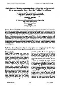
2 Kohonen Topological Map The Self-Organizing Map (SOM), proposed by Kohonen, is an unsupervised neural network. It projects high-dimensional data onto a lowdimensional map [14]. Such projection preserves the topological relationship defined into the data space; therefore, this ordered map can be used as a convenient visualization surface for showing various features of the training data. For example, cluster structures [13]. The Kohonnen network has one single layer. It called the output layer. The additional input layer just distributes the inputs to output layer. The neurons of this latter are arranged in a matrix (Fig. 1). The number of neurons on input layer is equal to the dimension of input vector. Kohonen has proposed various alternatives for the automatic classification [14], and presented the Kohonen topological map. The Kohonen model calculates the Euclidean distance between input data x and weights w .

3 Continuous Hopfield Network Hopfield neural network was introduced by Hopfield and Tank [11]-[12]. It was first applied to solve combinatorial optimization problems. It has been extensively studied, developed and has found many applications in many areas, such as pattern recognition, design systems [18], and optimization [9]. The Continuous Hopfield Networks (CHN ) consists of interconnected neurons with a smooth sigmoid activation function (usually a hyperbolic tangent function). The differential equation which governs the dynamics of the CHN as follows:

g (w, x) =P w x P

dy y = Tv I b (1) dt where y , v and I b are, respectively, the vectors

Fig.1. Kohonen topological map The structure of the Kohonen topological map can be defined graph in which the neurons represent the nodes. Basing on this structure, Kohonen has defined the discrete distance . For any pair of neurons ( g , i) , it calculate a discrete distance , where ( g , i) is defined as the length of the shortest path between g and i on the graph. For each neuron g, this discreet distance can be defined the concept of a neighborhood as follows: Vg = {i / ( g , i) d } , where d represents the ray of the neighborhood of the neuron g. Because of its effeteness in resolution of unsupervised learning problems, the SelfOrganizing Map (SOM) becomes a widely used method for data visualization. To improve this method, many variants and extensions have been

E-ISSN: 2224-2872

of neuron states, the outputs and the biases. The output function vi = g ( yi ) is a hyperbolic tangent, which is bounded below by 0 and above by 1. The real values Ti , j and I ib are, respectively, the weight of the synaptic connection from the neuron i to the neuron j and the offset bias of the neuron i . For y 0 IR n , a vector y e IR n is called an equilibrium point of the differential equation system (1) if: t e IR , t t e y (t ) = y e . Hopfield has introduced the energy function E on [0,1]n which is defined by:

156

Issue 4, Volume 12, April 2013

WSEAS TRANSACTIONS on COMPUTERS

E (v) =

1 t 1 v Tv ( I b )t v 2

n i =1

vi 0

M. Ettaouil, M. Lazaar, K. Elmoutaouakil, K. Haddouch

Since the objective function minimized by the Kohonen method doesn‘t contain any term which control the size of the map. The last one contains same unnecessary neurons. These neurons have a negative effect because they make the learning process heavier. Moreover, they make the labeling phase more difficult. To overcome this problem, we propose, in this paper, a new model that controls the size of the map, the geometrical error and conserves the notion of neighborhood which is defined in the observations set. In this section, we well describe the construction steps of our model. The first one consists in integrating the special term which control the size of the map. The second step gives the constraints which ensure the allocation of each data to only one neuron. Finally, we give the constraints that avoid the allocation of some data to removed neurons.

g 1 ( z )dz

It should be noted that if the energy function (or Layapunov function) exists, the equilibrium point exists too. Hopfield proved that the symmetry of weight matrix is a sufficient condition for the existence of Lyapunov function [11]. In order to solve combinatorial problems using CHN, we will write it in form of the energy function E (v) such that: E (v) =

1 t v Tv ( I b )t v 2

(2)

The extremes of this function are among the corners of the n-dimensional hypercube H = [0,1]n [10]-[17]. The philosophy of this approach is that the objective function, which characterizes the combinatorial problem, is associated with the energy function of the network when . In This way, the output of the CHN can be represented as a solution to combinatorial problem. Unlike a discrete network with the signum (hard-limiter) activation function, an analog neural network (with sigmoid activation function with variable slope) permits to avoid sub-optimal local minima. Moreover, the analog network is much faster and more reliable than the discrete neural network with an asynchronous update [1]-[16]. To ensure the feasibility of the equilibrium points of the CHN, some authors propose two steps (hyperplane method) [20]. The first one involves the decomposition of the set of the non feasible solutions into appropriate subsets, based on the constraints of the General Knapsack Quadratic Problem. In the second step, the parameters of the function are selected using the analytical conditions of the equilibrium points. The generalization of the energy function and these steps were used to solve the Salesman Traveling Problem [20], the Job Shop Scheduling Problem [7] the Graph Coloring Problem [20] and the Placement of the Electronic Circuit Problem [8]. Within these papers, the feasibility of the equilibrium points of the CHN is always guaranteed.

3.1 Assignment and decision variables The relationships between the data and the neurons of the map are governed by the following assignment variables:

Where i = 1,..., n , j = 1,..., N , n is the number of data and N is the number of neurons. To control the size of the topological map we use the following decision variables. 1, 0,

u0, j =

if the j th neuron is used . if the j th neuron is deleted .

3.2 Objective function This shout out a field of influence around each neuron of this map, we define the matrix R which called the neighborhood matrix: ( j, l ) ), T

R j ,l = exp(

j, l = 1,..., N

( j , l ) is a distance between the neuron j and the

neuron l . By doing this, we obtain the following cost function : n

N

N

ui , j R j ,l u0,l P xi

w j P2

u0, j

i =1 l , j =1

j =1

So that the neurons used will be consecutive, to avoid, a situation in which the neurons of a 4-class map can be constructed by 1, 8, 5 and 3, the variables x j can be penalized with the value q j in the objective function:

4 A new optimization model of the Kohonen architecture maps The philosophy of the Kohonen method consists of projecting the observations set into another space of a small dimension and, at the same time, conserve the notion of the neighborhood defined on the observations set. These conservations are realized by using the kernel function. So, the Kohonen method is a generalization of the Forgy method [5].

E-ISSN: 2224-2872

1 if the i th data assigned to j th neuron. 0 else

ui , j =

n

f (u, w) =

N

ui , j R j ,l u0,l P xi

w j P2

N

qu

i =1 j 0, j

i =1 l , j =1

The ( q j ) j must be an increasing sequence: 0 < q1 < ... < q j < q j

157

1

< ... < qN

Issue 4, Volume 12, April 2013

WSEAS TRANSACTIONS on COMPUTERS

M. Ettaouil, M. Lazaar, K. Elmoutaouakil, K. Haddouch

can be chosen between certain bounds in data function. The modeling of a variety of decision problems in areas such as the optimization neural architecture problems, usually leads to solve non linear mixedinteger problems. Most of these problems involve objective function expressed in the polynomial functions form. We can apply the technique of linearization or duality method for obtaining polynomial mixed-integer problem with constraints. The pertinent work indicates that basically two approaches are employed in solving polynomial mixed-integer problems; namely, exact methods and heuristic methods. The present paper falls in the latter group, because the linearization procedures suffer from the increase of the variables and constraints number and the duality methods needs extremely high iterative computing for training. In this mean, we use the Continuous Hopfield Networks (CHN) to solve the proposed mixedinteger problem (P).

3.3 Constraints The following family of constraints guarantees that the assignment of each example to only one neuron: N

ui , j = 1,

(3)

i = 1,..., n

j =1

When the neuron j is not used, the variable ui , j must take the value 0. To this end, the following quadratic constraint must be added as a new constraint: N

n

(1 u0, j ) j =1

(4)

ui , j = 0 i =1

This constraint can be called "the transmission constraint", because it allows to transmit the information from the variables u0, j to the variables ui , j .

3.4 Optimization model To Tak into consideration the cost function, the allocation constraints and the transmission one, we obtain the following model which optimizes the number of used neurons and conserve, at the same time, the notion of neighborhood defined on the observations set: n

N

Min

5 A new training algorithm based on the CHN and the proposed model In this section, we use the Continuous Hopfield Networks (CHN) to solve the problem (P). Since the problem (P) is a mixed-integer problem with a polynomial objective function, we will solve it basing on two steps: - Assignment phase: we fix the weight vectors and we solve the obtained problem: the polynomial assignment problem of integer variables. - Minimization phase: we fix the assignment vectors and we solve the obtained problem: the non linear optimization problem with continuous variables. First, the weights are initialized as follows: The vector weights are, randomly, initialized from the set DS = mp =1[ xmmin , xmmax ] . xmmax = max{xmi / i = 1,..., n} where and min i xm = min{xm / i = 1,..., n} , m =1,..., p . This choice can be justified by the fact that all the observations are in the Data. Moreover, we can prove theoretically that the weights associated with an optimal solution are in the Data.

N

ui , j R j ,l u0,l P x

i

j

2

w P

i =1 l , j =1

q j u0, j j =1

SC : N

ui , j = 1

( P)

i = 1,..., n

j =1 N

n

(1 u0, j ) j =1

ui , j w

j

ui , j = 0 i =1

{0,1} i = 0,..., n IR

p

j = 1,..., N

j = 1,..., N

We define the vectors u and q as follow: u = (u0,1 ,..., u0, N , u1,1 ,..., u1, N ,..., ui, j ,..., un, N )t q = (q1 ,..., qN )t

IR N

Let (u*, w*) be an optimal solution of the mixed integer problem (P), we can prove, theoretically, that the introduction of the second term in the objective function prevented the number from tending to N . Several algorithms have been proposed to solve MINLPs: Branch-and-Bound, Outer Approximation, LP / NLP -based Branch-andBound, and Branch-and-Cut. In this part, a new optimization model is introduced. In order to optimize the architecture of the topological map (select the optimal number of the neurons in the map) and adjust the weights matrix (learning), the number of neurons in the map

E-ISSN: 2224-2872

5.1 The continuous Hopfield network architectures for the assignment phase At the iteration t , we fix the weight vectors obtained in the iteration (t 1) and we solve the following optimization problem with integer variables using the CHN:

158

Issue 4, Volume 12, April 2013

WSEAS TRANSACTIONS on COMPUTERS

n

N

M. Ettaouil, M. Lazaar, K. Elmoutaouakil, K. Haddouch

N

ui , j R j ,l u0,l P x i

Min

w j P2

E0,b (u) = E (u) / u0,b =

q j u0, j

i =1 l , j =1

j =1

qb

SC : ( Pt )

ui , j = 1, i = 1,..., n N

C

n

hC (u ) =

(1 u0, j ) j =1

ui , j = 0

N ( n 1)

H F = {u {0,1}

/

C

h (u ) = 0 and

ei (u ) = 1, i = 1,..., n}

C

hC (u ) N

0

N

C

u RbT,l P x a

l =1 0,l N

u0,b

u

j =1 a , j

1

wb (t 1) P2 (1 2ua ,b )

>0

To solve the problem ( Pt ) using the CHN a suitable energy function must be constructed:

C

(1 2u0,b )

On the other hand, to penalize the nonfeasibility of the quadratic constraints hC (u ) and the family of linear constraints ei (u ) , it is natural to impose the constraint that:

- Energy function for the problem ( Pt )

i =1

0

w j (t 1) P2

To minimize the objective function, we impose the following constraint:

The feasible solutions set of the problem ( Pt ) is:

E (u ) = (

u

i =1 i ,b

u RTj ,b P xi

i =1

IR p , j = 1,..., N

n

j =1 i , j

Ea,b (u) = E (u) / ua ,b

j =1

wj

N

For a = 1,..., n and b = 1,..., N

N

ei (u ) =

n

C

n i =1

N

u R u Px l , j =1 i , j j ,l 0,l 1 2

n

i

j

w P n

[ei (u)]2

u (1 u0, j )

1

qu ) j =1 j 0, j

e (u )

i =1 i

i =1

j =1 0, j

0. So that the instability of the interior points u H HC is guaranteed, some initial conditions are imposed on some parameters: T0b,0 d = 2 0 0 , b = 1,..., N and d =1,..., N Tab, cd = 2 1 0 for a =1,..., n, c =1,..., n , b = 1,..., N , and d =1,..., N Given the two types of constraints:

N

2

N

n

j =1

i =1

(1 ui , j )ui , j

Taking into account that u is the neuron output of the CHN, I is the bias of the network and T is the weights matrix of the connection in the network

0,

ei (u) = 1

1 t with energy function v Tv ( I b )t v , the weights of 2 the connections between the (n 1) N neurons are:

i = 1,..., n

C

h (u ) = 0

The partition of H C H F is defined as: - H = {hC (u ) > 0} . In this case, there exist some observations xa have been assigned to a non used neuron b , this means that u0,b = 0 and ua ,b = 1 ; consequently, u0, j must be increased so that the partial derivative E0,b (u ) > . To guarantee this, and taking into account that (qb ) is an increasing sequence, the following condition is imposed: C . 1 1,1

T0b,0 d = 2 b, d . 0 T0 d , ab = Tab,0 d = RbT, d P x a Tab ,cd = ( 2 1 ) a ,c . b,d I 0, j = .qb 0 C I a ,b = 1

Where a = 1,..., n , d =1,..., N .

wb (t 1) P2

b = 1,..., N ,

C

.

b, d

(5)

c = 1,..., n

and

-

- Parameter setting

n

H 3,1 = {hC (u) = 0} {i =1{ei (u) > 1}} . In this

way, one observation xa has been assigned two different neurons b and d so that ua ,b = ua , d = 1 . As in the previous case, the value u a ,b will decrease if Ea ,b (u ) .

A feasible solution is guaranteed by the CHN from a stability no linear analysis of the Hamming hypercube corners set: H C = {0,1}N ( n 1) . The parameter-setting procedure is based on the partial derivatives of the generalized energy function: For b = 1,..., N

Taking into account that hC (u ) = 0 and ua ,b = 1 , then u0,b = 1 in such a way that the following constraint is obtained: ( M 2t

1

qN )

C

where

E-ISSN: 2224-2872

159

Issue 4, Volume 12, April 2013

WSEAS TRANSACTIONS on COMPUTERS

M 2t 1 = max b{

- H

n

N

i =1

j =1

RTj ,b P xi

M. Ettaouil, M. Lazaar, K. Elmoutaouakil, K. Haddouch

n

w j (t 1) P2 } n

C

Where k = 1,..., n . So, there is misclassified observation xa , this means that a such that ua ,b = 0 , b = 1,..., N and therefore the value u a , b . will increase if Ea ,b (u ) The following constraint is a sufficient condition to get Ea ,b (u ) : M 1t

where

M

N

= max a,b{

R Px

a

b

2

1

0, 0,

1

j =1

ui , j

2

w (t 1) P } ,

I u (w) =

( M 2t

M 1t

1

0; C

;

n

N

i =1

l , j =1 i , j

n

u R j ,l u0,l P xi

N

w j (t ) = (

1

N a ,b

RbT,l P x a

qu

j =1 j 0, j

is

n

N

RTj ,l ui , j u0,l )

(8)

i =1 l =1

j at the iteration t . N

= max{

R

T j ,b

Px

i

j

2

w (t 1) P }

5.3 Training algorithm

(6)

Basing on the equations (5), (6), (7), (8), and on the algorithm presented in [19], we propose the following learning algorithm:

i =1 j =1

Input: • n , p , x1 ,..., xn ; • [Tmin , Tmax ] ; the interval of the parameter T; • , , 1 , N iter ; Output: Optimal topological map Initialization: • N the size of the map • w1 (0),..., wN (0) ; randomly initialized • T Tmax , t 0 ; Repeat assignment-decision phase Calculate M 1 and M 2 via the equation (6); Calculate C , , and 1 via the equation (7); Calculate T and I via the equation (5); Calculate the equilibrium points of the CHN via the Euler method; minimization Phase; while( j < N ) do if( u0, j 0 ) then update the weight w j via the equation (8);

Where b = 1,..., N and a = 1,..., n . A feasible solution could be the following: > 0, 1 0, > 0, 0 = 0 =2 1 c = max(2 M 1t 1 , M 2t t 1 = M1 1

1

qN

)

(7)

Given the size of the description space and the size of the Kohonen topological map, we can determine the parameters by resolving the later System (7).We need to fix , and compute the other parameters.

5.2 Minimization phase In this step, we fix the variables vector u , and we solve the following optimization problem with continuous variables:

E-ISSN: 2224-2872

N

w j (t ) represents the gravity center of the class

wb (t 1) P2 }

l =1 n

b

w j P2

RTj ,l ui , j u0,l xi ) / ( i =1 l =1

M 1t 1 = max{

Where M

j = 1,..., N

Since it is sufficient to ensure that in every iteration, we use only a simple gradient method:

1

t 1 2

IR p

Iu (w) / w = 0

; qN )

{0,1} i = 0,..., n

a convex quadratic function, the solution of the problem ( Pu ) is given by the following system:

C 1

j

ui , j = 0 i =1

As

>0; 0

n

(1 u0, j )

with b = 1,..., N and a = 1,..., n . We can summarize it as following: >0,

ui , j = 1 j =1

w T l =1 b,l

q j u0, j j =1

N

(Pu )

1

N

w j P2

SC :

1

t 1 1

N

ui , j R j ,l u0,l P x i i =1 l , j =1

= {h (u) = 0} {ek (u) 1} {i =1{ei (u) = 0}}

3,2

N

Min

160

Issue 4, Volume 12, April 2013

WSEAS TRANSACTIONS on COMPUTERS

M. Ettaouil, M. Lazaar, K. Elmoutaouakil, K. Haddouch

proposed model. Because of this proposed model, the number of neurons decreases with time. Finally, we show that, the unnecessary units are dropped from the map.

endIf t

t 1; t

T

j

T N Tmax ( min ) iter Tmax

1

;

TABLE 1 COMPUTING THE OPTIMAL NEURONS OF THE MAP USING

j 1;

THE PROPOSED METHOD

done Until[ ( t < Niter ) )OR ( Min P w j (t ) w j (t 1) P> 1 )] return (The optimal topological map and final weights);

initial size 25 36 42 50 64 70 80 90

Algorithm 1: Optimal Kohonen topological map This method is based on the well known Nues Dynamique method. The Nues Dynamique method will converge if the cost fulfils some criteria [5], this algorithm ensures that the function of the cost converge to a local minimum; what's more, the choice of the initial weights has a great effect on the convergence of the proposed algorithm.

nbr. iteration 150 150 130 130 120 120 100 100

optimal size 10 12 11 10 11 12 13 11

The TABLE 1, present in the mean of the remaining neurons associated with different size of maps and different iterations. So, the necessary number of neurons to clusters data IRIS converges approximatively to 11 neurons.

6 Computational experiments Many different approaches have been used in order to classify the three components of data Iris[23]. In order to point out the advantages of the optimization Kohonen architectures, we apply our algorithm to a widely used dataset: Iris dataset for classification. It consists of three target classes: Iris Setosa, Iris Virginica and Iris Versicolor. Each class contains 50 data samples. Each sample has four real-valued features: sepal length, sepal width, petal length and petal width. Before training, data are normalized using the following rule: xki new =

xki old min( xi ) max( xi ) min( x i )

(9) Fig. 2. Necessary units versus iterations

The half of the data samples are used for training and 75 items for testing. It should be noted that we have used only a small number of the data to label the neurons of the map because the last one is controlled by the proposed model. The parameters , , 0 and q j of the CHN are sitting as follows: = 0.001 , 1 = 0.5 , =10 4 , nj ) . 0 = 0 and q j = jn / ( N

The numerical results are presented in Fig. 2. For example for a map contains 42 neurons, the mean of remaining neurons is approximately 11 neurons in 130 iterations. The proposed method completes the Kohonen learning method. In fact, our approach releases two tasks at the same time: the learning task and the optimization one which consists minimizing the size of the map. These goals are achieved in three phases: Allocation phase, decision phase and the minimization one. By this one, we get at the convergence only the useless neurons and labialization task becomes easy. The TABLE 2 presents the obtained clustering results of training data. This table shows that our method gives the good results, because all the training data were correctly classified except two. In fact; these elements (misclassified) are from the Versicolor class.

The parameters , C , 1 and are calculated using the equations (6) and (7). The outputs of the network CHN are initialized as follows: ui , j = b.(i j ) / ( N (n 1) i j ) . With i = 0,..., n and j = 1,..., N To cluster data IRIS, the initial size of the map is randomly choosing; this size is controlled by the term q j u0, j in the objective function of the

E-ISSN: 2224-2872

TABLE 2

161

Issue 4, Volume 12, April 2013

WSEAS TRANSACTIONS on COMPUTERS

M. Ettaouil, M. Lazaar, K. Elmoutaouakil, K. Haddouch

NUMERICAL RESULTS FOR CLUSTERING THE TRAINING

product the good classification than the other method; but our method gives less time than EBP (9.5 seconds). These good results can be argued as follows: - The first term of the objective function of our proposed model controls the geometric error on a given classification. - To facilitate the task of labialization the kernel matrix ensures the conservation of the topology of data space and that the creation of a field of influence of each neuron. - The second term of the objective function keeps only the neurons that represent the reel density of data. - The fastness of our method is the using of Hopfield network in the allocation phase. In addition, the number of hidden neurons must be decided before training in both EBP and RBF neural networks. Different number of hidden neurons results in different training time and training accuracy. It is still a difficult task to determine the number of hidden neurons in advance. The experiments indicated that clustering by the proposed method is computationally effective approach.

DATA

Setosa Virginica Versicolor Total

Nbr. Tes.D Cr.Class MC Accuracy (%) 25 25 0 100 25 25 0 100 25 23 2 92 75 73 2 97.33

The TABLE 3 shows the numerical results obtained from the data classification of the testing data. We see that, the important results are obtained because we have, only, two misclassified data among 75 testing data. These misclassified data belong to Versicolor class. TABLE 3 NUMERICAL RESULTS FOR CLUSTERING THE TESTING DATA Nbr. T. D Cr.Class MC Accuracy (%) Setosa 25 25 0 100 Virginica 25 25 0 100 Versicolor 25 23 2 92 Total 75 73 2 97.33

‐ Nbr. T. D. is Number of Training Data, ‐ Cr.Class. is Correctly Classified. ‐ MC. is Misclassified The weights initialization of the Kohonen algorithm and the fixation of the neural architecture by the proposed method demonstrate the important impact: The final partitioning was done by the following procedure. - Weights initialization of the Kohonen algorithm and the fixation of the neural architecture; - A SOM was trained using the sequential training algorithm for each example of training data.

7 Conclusion In this paper, we have modeled the selection of the Kohonen architecture in terms of a mixed-integer optimization problem with non linear constraints. This new model optimizes the Kohonen network architecture and, at the same time, conserves the notion of the neighborhood defined on the observation set. Basing on this model, we have proposed a learning classification method by giving a learning rule in the minimization phase; because of its effectiveness in solving the optimization problems, the Continuous Hopfield Network (CHN) is used in the assignment-decision phase. In comparison with the classical learning method of Kohonen, the proposed method is able to avoid the unusless neurons in the map. The experimental work for classification problems has illustrated the advantages of proposed approach, especially in the quality of the classification and in the optimization of the architecture map. In order to point out the advantages of the proposed approach, we have applied the proposed algorithm to a widely used dataset, Iris dataset for classification. In this respect, the proposed method produces a good classification, in reasonable time, in comparison with the recent methods like EBF, RBF and SVM. In the future, we will use the proposed method for the image compression and speech processing.

TABLE 4 COMPARISON FOR IRIS DATA CLASSIFICATION Methods CPU(s) It. M.T. M.TS. A.T. A.TS. EBP 39.98 500 3 2 96 97.3 EBP 68.629 800 2 1 97.3 98.6 RBF 16.84 85 4 4 94.6 94.6 RBF 19.81 111 4 2 96 97.3 SVM 8.743 5000 3 5 94.6 93.3 P.M. 9.5 150 2 2 97.3 97.3

‐ ‐ ‐ ‐ ‐

It : Number of iterations; M.T. : Misclassified for training set; M.TS. : Misclassified for testing set; A.T. : Accuracy for training set; A.TS. : Accuracy for testing set. ‐ P.M. is the Proposed Method From the TABLE 4, it is clear that our method gives the good results, in comparisons with the other ones, RBF, EBP and SVM. In one hand, SVM method gives a less time than our approach, but our approach gives a good classification (4 misclassified). In the other hand, EBP method gives

E-ISSN: 2224-2872

162

Issue 4, Volume 12, April 2013

WSEAS TRANSACTIONS on COMPUTERS

M. Ettaouil, M. Lazaar, K. Elmoutaouakil, K. Haddouch

[12] J.J. Hopfield, ―Neurons with graded response have collective computational properties like those of two-states neurons‖, proceedings of the National academy of sciences of the USA 81, pp. 3088-3092, 1984. [13] J.J. Hopfield, D.W. Tank, ―Neural computation of decisions in optimization problems‖, Biological Cybernetics 52, pp. 1-25, 1985. [14] C. C. Hsu, ―Generalizing Self-Organizing Map for Categorical Data‖, IEEE Transactions on neural networks, Vol. 17, No. 2, pp. 294-304, 2006. [15] T. Kohonen. ―Self Organizing Maps‖. Springer, 3e edition, 2001. [16] B.W. Lee, B.J. Shen, ―Hardware annealing in electronic neural networks‖, IEEE Trans, Vol. 1, pp. 134 -137, 1990. [17] N.M. Nasrabadi and C.Y. Choo, ―Hopfield network for stereo vision correspondence‖, New York:Marcel Dekker, 1994. [18] H. Shah-Hosseini, R. Safabakhsh. ―TASOM: The Time Adaptive Self-Organizing Map‖. International Conference on Information Technology: Coding and Computing (ITCC'00), 422, 2000. [19] P.M. Talaván and J. Yàñez, ―A continuous Hpfield network equilibrium points algorithm‖. Computers and operations research, Vol. 32, pp. 2179-2196, 2005. [20] P.M. Talaván, J. Yàñez, ―The generalized quadratic knapsack problem.A neuronal network approach‖, Neural Networks, Vol. 19, pp. 416-428, 2006. [21] D. Wang. N.S. Chaudhari, ―A constructive unsupervised learning algorithm for Boolean neural networks based on multi-level geometrical expansion‖, Neurocomputing, 57C: pp. 455-461, 2004. [22] H. Yin, ―ViSOM—A Novel Method for Multivariate Data Projection and Structure Visualization‖, IEEE Transactions on Neural Networks, Vol. 13, pp. 237-243, 2002. [23] www.ics.uci.edu/mlearn/MLRepository.html.

References: [1] S.V.B. Aiyer, M. Niranjan, and F. Fallside, ―A theoretical investigation into the performance of the Hopfield model‖, IEEE Trans. Neural Networks, Vol. 1, pp. 204-215, 1990. [2] N. Arous, N. Ellouze, ―Study of Specific Genetic Operators for Learning Kohonen Maps in Function of Initial Conditions‖, International Review on Computers and Software (IRECOS), Vol. 3. n. 6, pp. 610 – 617, November 2008. [3] W. Bellil, C. Ben Amar, A. M. Alimi, ―Multi Library Wavelet Neural Network for Lossless Image Compression‖, International Review on Computers and Software (IRECOS), Vol. 2. n. 5, pp. 520 – 526, September 2007. [4] Bouktir, T., Slimani, L., Optimal power flow of the Algerian Electrical Network using genetic algorithms, Wseas Transactions On Circuits And Systems, Vol. 3, Issue 6, 2004, pp. 14781482. [5] G. Dryfus, J.M.Martinez, M.Samuelides, M.B.Gordan, ―Réseaux de neurones Méthodologie et applications‖. EYRLLES, SC 924, 2000. [6] M. Ettaouil, Y.Ghanou, K. Elmoutaouakil, M. Lazaar, ―A New Architecture Optimization Model for the Kohonen Networks and Clustering‖, Journal of Advanced Research in Computer Science (JARCS), Vol. 3, Issue 1, pp. 14 - 32, 2011. [7] M. Ettaouil, K. Elmoutaouakil and Y. Ghanou, ―The Continuous Hopfield Networks (CHN) for the Placement of the Electronic Circuits Problem‖, Wseas Transactions On Computer, Issue 12, Volume 8, 2009. [8] M. Ettaouil, K. Elmoutaouakil, Y.Ghanou, ―The continuous hopfield networks (CHN) for the placement of the electronic circuits problem‖, Wseas Transactions on Computer,Vol. 8 Issue 12, December 2009. [9] M. Ettaouil and C. Loqman, ‗Constraint satisfaction problem solved by semi definite relaxation‘, Wseas Trasactions On Computer, Issue 7, Volume 7, 951-961, 2008. [10] D. J. Evansi and M. N. Sulaiman, ―Solving optimization problems using neucomp-a neural network compiler‖, International Journal of Computer Mathematics, Vol. 62, pp. 1-21, 1996. [11] A. Ghosh, S.K. Pal, ―Object Background classification using Hopfield type neural networks‖, International Journal of Pattern Recognition and artificial Intelligence, pp. 9891008, 1992.

E-ISSN: 2224-2872

163

Issue 4, Volume 12, April 2013