A comprehensive simplex-like algorithm for network optimization and

This article was downloaded by: [University of Illinois at Urbana-Champaign] On: 21 August 2013, At: 22:10 Publisher: Taylor & Francis Informa Ltd Registered in England and Wales Registered Number: 1072954 Registered office: Mortimer House, 37-41 Mortimer Street, London W1T 3JH, UK

Optimization: A Journal of Mathematical Programming and Operations Research Publication details, including instructions for authors and subscription information: http://www.tandfonline.com/loi/gopt20

A comprehensive simplex-like algorithm for network optimization and perturbation analysis a

H. Arsham & M. Oblak

a

a

Information and Quantitatice Sciences, Uniuersity of Baltimore, Baltimore, MD, 21201-5779, USA Published online: 20 Mar 2007.

To cite this article: H. Arsham & M. Oblak (1995) A comprehensive simplex-like algorithm for network optimization and perturbation analysis, Optimization: A Journal of Mathematical Programming and Operations Research, 32:3, 211-267, DOI: 10.1080/02331939508844049 To link to this article: http://dx.doi.org/10.1080/02331939508844049

PLEASE SCROLL DOWN FOR ARTICLE Taylor & Francis makes every effort to ensure the accuracy of all the information (the “Content”) contained in the publications on our platform. However, Taylor & Francis, our agents, and our licensors make no representations or warranties whatsoever as to the accuracy, completeness, or suitability for any purpose of the Content. Any opinions and views expressed in this publication are the opinions and views of the authors, and are not the views of or endorsed by Taylor & Francis. The accuracy of the Content should not be relied upon and should be independently verified with primary sources of information. Taylor and Francis shall not be liable for any losses, actions, claims, proceedings, demands, costs, expenses, damages, and other liabilities whatsoever or howsoever caused arising directly or indirectly in connection with, in relation to or arising out of the use of the Content. This article may be used for research, teaching, and private study purposes. Any substantial or systematic reproduction, redistribution, reselling, loan, sub-licensing, systematic supply, or distribution in any form to anyone is expressly forbidden. Terms & Conditions of access and use can be found at http://www.tandfonline.com/page/terms-and-conditions

Optimization, 1995, Vol. 32, pp. 21 1-267 Reprints available directly from the publisher Photocopying permitted by license only

C 1995 OPA (Overseas Publishers Association) Amsterdam BV. Published under license by Gordon and Breach Science Publishers SA. Printed in Malaysia

A COMPREHENSIVE SIMPLEX-LIKE ALGORITHM FOR NETWORK OPTIMIZATION AND PERTURBATION ANALYSIS

Downloaded by [University of Illinois at Urbana-Champaign] at 22:10 21 August 2013

H. ARSHAM and M. OBLAK Information and Quantitatice Sciences Uniuersity of Baltimore, Baltimore, M D 21201-5779, USA (Receiued 13 December 1993; injinalform 23 May 1994) The family of network optimization problems includes the following prototype models: assignment, critical path, max flow, shortest path, and transportation. Although it is long known that these problems can be modeled as linear programs (LP), this is generally not done. Due to the relative inefficiency and complexity of the simplex methods (primal, dual, and other variations) for network models, these problems are usually treated by one of over 100 specialized algorithms. This leads to several difficulties. The solution algorithms are not unified and each algorithm uses a different strategy to exploit the special structure of a specific problem. Furthermore, small variations in the problem, such as the introduction of side constraints, destroys the special structure and requires modifying andjor, restarting the algorithm. Also, these algorithms obtain solution efficiency at the expense of managerial insight, as the final solutions from these algorithms do not have sufficient information to perform postoptimality analysis. Another approach is to adapt the simplex to network optimization problems through network simplex. This provides unification of the various problems but maintains all the inefficiencies of simplex, as well as, most of the network inflexibility to handle changes such as side constraints. Even ordinary sensitivity analysis (OSA), long available in the tabular simplex, has been only recently transferred to network simplex. This paper provides a single unified algorithm for all five network models. The proposed solution algorithm is a variant of the self-dual simplex with a warm start. This algorithm makes available the full power of L P perturbation analysis (PA) extended to handle optimal degeneracy. In contrast to OSA, the proposed PA provides ranges for which the current optimal strategy remains optimal, for simultaneous dependent or independent changes from the nominal values in costs, arc capacities, or supplies/demands. The proposed solution algorithm also facilitates incorporation of network structural changes and side constraints. It has the advantage of being computationally practical, easy for managers to understand and use, and provides useful PA information in all cases. Computer implementation issues are discussed and illustrative numerical examples are provided in the Appendix.

KEY WORDS: Linear network optimization, assignment problem, critical path, max flow, min flow, shortest path, transportation problem, perturbation analysis, sensitivity analysis, parametric sensitivity analysis, tolerance analysis. the 100% rule, linear program, self-dual simplex, more-for-less paradox, degeneracy, redundancy. Mathematics Subject Classification 1991: Primary: 90C34; Secondary: 90C20,90C25.

Table of Contents and Global Abbreviations 1. Introduction and Summary 1.1. Problem Statement and L P Formulations for Network Models 1.2. Difficulties with L P Formulation of Networks 1.3. Solution Algorithms for Network Models

212

H. ARSHAM AND M. OBLAK


1.4. Strategy for New Simplex-variant Algorithm 1.5. Network Perturbation Analysis (PA) 1.6. Network-based Approaches to PA 2. The Simplex-Like Network Algorithm 2.1. Preliminary Phase 2.1.1. Assignment Problem 2.1.2. Critical Path Problem 2.1.3. Max Flow Problem 2.1.4. Shortest Path Problem 2.1.5. Transportation Problem 2.2. Basic Variable Set (BVS) Augmentation Phase 2.3. Optimality (OP) Phase 2.4. Feasibility (FE) Phase 2.5. More-for-less (MFL) Identification and Solution for T P 2.6. Outline Proof of Algorithm 2.7. Computer Implementation Issues 2.7.1. Sparsity and Data Structure 2.7.2. The Push Phase 2.7.3. The Push Further and Pull Phases 2.7.4. Other Pivoting and Anti-cycling Strategies 3. Perturbation Analysis 3.1. Cost Perturbation Analysis 3.1.1. General Perturbation Set 3.1.2. Parametric Sensitivity Analysis (PSA) 3.1.3. Ordinary Sensitivity Analysis (OSA) 3.1.4. The 100% Rule 3.1.5. Tolerance Analysis (TA) 3.2. Arc Capacity Perturbation Analysis 3.2.1. General Perturbation Set 3.2.2. Parametric Sensitivity Analysis (PSA) 3.2.3. Ordinary Sensitivity Analysis (OSA) 3.2.4. The 100% Rule 3.2.5. Tolerance Analysis (TA) 3.3. Supply and Demand Perturbation Analysis 3.3.1. General Perturbation Set 3.3.2. Parametric Sensitivity Analysis (PSA) 3.3.3. Ordinary Sensitivity Analysis (OSA) 3.3.4. The 100% Rule 3.3.5. Tolerance Analysis (TA) 4. Managerial Implications and Concluding Remarks References Appendix: Illustrative Numerical Examples A. 1. Assignment Problem (AP) A.2. Critical Path Problem (CP) A.3. Max Flow Problem (MF) A.4. Shortest Path Problem (SP)

NETWORK OPTIMIZATION ANALYSIS

213

A.5. Transportation Problem (TP) A.6. Accessing Data via Link List 1. INTRODUCTION AND SUMMARY In this paper we are concerned with the solution and perturbation analysis of the following prototype network models: assignment, critical path, max flow, shortest path, and transportation. Perturbation analysis is invaluable in practice because problem data are often only approximate ( e g forecasted), and/or because we would like to understand how robust a solution is to change in the underlying data.


I .I

Problem Statement and LP Formulations for Network Models

This section provides a description and L P formulation for the classic network models. Assignment Problem (AP):Typically, we have a group of n "applicants" applying for n "jobs," and the cost C i j> 0 of assigning the ith applicant to jthjob is known. The objectiveis to assign onejob to each applicant in such a way as to achieve the minimum possible total cost. Define binary variables X i j with value of either 0 or 1.When X i j = 1, it indicates that we should assign applicant i to job j. Otherwise ( X i j= 0), we should not assign applicant i to job j. Formally, we have: n

Min

n

1 1C i j X i j

subject to: n

X i j = 1, for j = 1,.. . n (Each job is assigned to one applicant)

i= 1

n

X i j = 1, for i = 1,.. . n (Each applicant is assigned to one job). j= 1

In any optimal solution exactly n of the 2n - 1 basic variables have value 1 and (n non-basic variables have value 0. Thus, AP as a L P is extremely (primal) degenerate, which causes additional difficulties with L P sensitivity analysis. In fact, in several computational studies it was observed that when solving large problems by the standard simplex, 95 percent of the pivots are degenerate [58]. The PA deals with the range of values for the assignment cost C i j for which the current optimal assignment remains optimal. Among related problems are: The 1-matching and B- matching problems, the three-dimensional AP, and the bottleneck AP, more details are given in [13,96]. Critical Path Problem (CP): Given a network of activities, the problem of interest is to determine the length of time required to complete the project and the set of critical activities which control the project completion time. Suppose that in a given project activity network there are m nodes, n arcs (i.e. activities) and an estimated duration time, Cij,associated with each arc (i + j) in the network. The beginning node of an arc corresponds to the start of the associated activity and the end node to the completion of an activity. To find the CP, define the binary variables Xij, where X i j = 1 if the activity i-, j is on the C P and X i j = 0 otherwise. The length of the path is the sum of the

H. ARSHAM A N D M. OBLAK

214

durations of the activities on the path. The length of the longest path is the shortest time needed to complete the project. Formally, the C P problem is to find the longest path from node 1 to node m. m

Max

m

1 CijXij

i = l j=1

subject to:

x m


-

Xij +

j= 1

x m

Xki= 0, for i # (1 or m)

k=l

where the sums are taken over existing arcs in the network. The first and the last constraints are imposed to find the critical activities that start (node 1)and complete the project (node m) respectively, while the other constraints impose the criterion that if you enter a node by a critical activity you must leave that same node by a critical activity. The PA deals with the range of values for the duration times Cij for which the set of critical activities remains the same. Maxiinum $ow problem (MF): In a network with flow capacities on the arcs, the problem is to determine the maximum possible flow from the source to the sink while honoring the arc flow capacities. Consider a network with m nodes and n arcs with a single commodity flow. Denote the flow along arc (i-, j) by fij. We associate with each arc a flow capacity, kij. In such a network, we wish to find the maximum total flow in the network, f , from node 1 to node m. Max f subject to: rn fij j= 1

1

k=l

fki =

[ f , i f i = l O, if i # (1 or m) -f, if i = m

The sums and inequalities apply over existing arcs in the network. The equality constraints state that the total flow into the node must equal the total flow out of the node for every node in the network, including the source and the sink nodes. The PA determines how much the arc capacities, kij, can be changed while ensuring that the maximum flow route remains optimal. A closely related problem to M F is the minimum flow (MIF) problem, see e.g. [ 2 ] . Assume that fij is the flow and wij is the lower bound on flow associated with each -c (i -* j) in the network. Let node 1 be the source node and node m the sink node. Then


215

the MIF problem is [I]: Min f subject to


f i j2

wij, for all i, j,

where the sums are taken over existing arcs in the network. Note that one of these equality constraints is redundant (e.g. the last constraint is the sum of all other constraints). Lower flow bounds wij can be changed to zero by a translation of variables, that is by replacing Sij = f i j - wij. Since there is a lower bound wij on the flow of each arc, we denote the excess capacity used on arc (i -+ j) as a non-negative surplus variables Sij such that Sij= Lj - wij.The equivalent problem is: m

1S l j

Min

i=l

subject to

1Sik- 1Skj= C wkj- 1wik, i=l

J=

1

j= 1

for k # 1 or m all Sij 2 0.

i= 1

Note that the MIF is completely formulated in terms of surplus variables Sip There would be at most m-2 over-flows, m being the number of nodes. The optimal flows and the optimal value of the original problem are obtained by adding Sijto the optimal flow for each arc and adding I S , , to the optimal value of the transformed problem. This saves computational time and storage and for this reason most network flow codes assume that the lower flow bounds are zero. For detailed postoptimality of the M I F see [I]. Shortest path problem (SP): The problem is to determine the best way to traverse a network to get from an origin to a given destination as cheaply as possible. Suppose that in a given network there are m nodes and n arcs and a cost Cijassociated with each arc (i + j ) in the network. Without loss of generality we assume Cij 2 0. Formally, the SP problem is to find the shortest (least cost) path from the start node 1 to the finish node m. The cost of the path is the sum of the costs on the arcs in the path. Define binary variables Xij, where Xij = 1 if the arc (i + j ) is on the SP and Xij = 0 otherwise. m

m

1 2 CijXij

Min subject to:

-

m

m

j= 1

k=l

2 Xij + C Xki= 0

for i # (1 or m)


216


where the sums are taken over existing arcs in the network. The first and the last constraints are imposed to force a path from the start node (node 1) to the finish node (node m) respectively, while the other constraints ensure that the path does not remain at any intermediate nodes. The PA is concerned with how much the arc costs Cijcan be changed while making sure that the current shortest path remains optimal. Although this problem is similar to CP, the longest path problem, they have two primary distinct fields of application, namely project management [I51 for C P and communication networks [I41 for SP. Therefore, we consider each separately. Transportation problem (TP): A shipper having m warehouses with supply ai of goods at his ithwarehouse must ship goods to n geographically dispersed retail centers, each with a given customer demand ej which must be met. The objective is to determine the minimum possible transportation costs given the unit cost of transportation between the ithwarehouse and the jthretail center is Cij. Formally T P is defined as: m

Min

n

1 CijXij

i = l j=1

subject to: n

1X i j = a i

for i = 1,2, ...,m

j= 1 m

X i j = e j for j = 1,2,...,n. i=l

The PA asks how much supplies (a,),demands (ej) and/or shipment costs (Cij)can be changed while making sure that the current shipment route remains optimal. A second important use of PA for T P is in the paradoxical more-for-less (or nothing) situation (MFL). The MFL (nothing) situation can be stated as follows: given an optimal solution, it is possible to ship more total good for less (equal) total cost even if at least the same amount is shipped from each origin and to each destination, and all the shipping costs are non-negative. Such information is useful to a distribution manager in deciding which warehouse capacities are to be increased, and which markets should be sought after. Here, PA finds the maximum additional shipments and its distribution in a systematic way. Arsham [16] suggests combining the MFL problem and the perturbed supply/demand TP as follows: m

n

1 1 CijXij

Min

i = l j=1

subject to:

1 Xij-ri=ai,

for i = 1 , 2 ,...,m

j= 1

m

Xij - kj = ej, for j = 1,2,. . . , n. i=l

xij3 0,

r, 3 0, and kj 3 0.

We follow this approach in this paper.


217

These five prototypes are simple and classical applications of network models. There are many indirect, wide-ranging, practically important applications of these models. See the bibliography in Ahuja et al. [4] containing over 200 diverse and interesting real-world applications. Although some of these problems are somewhat similar in their L P formulation, such as C P and SP, they are sufficiently important to be considered separately. The proposed algorithm is designed in such a way to handle a very general class of network problems. The generalized problem is as follows: m

Min

m

C 1CijXij i = l j=l

subject to: Downloaded by [University of Illinois at Urbana-Champaign] at 22:10 21 August 2013

m

m

+ 1 bkiXki= di

aijXij j= 1

for i = 1,2,. . . ,m

k= 1

0 < xij< Uij,

for all i, j,

where the sums are taken over existing arc in the network. This problem differs from the models we outlined above in that the nonzero entries in the coefficient matrix may be different from 1. This generalization also allows, for example a specified gain or loss (d,) at each node [25]. Furthermore, it is not a requirement that the nonzero entries in the coefficient matrix must have an opposite sign, as in the Generalized Network Problem, see e.g., [40,107].

+

1.2 DifJiculties With LP Formulation of Networks

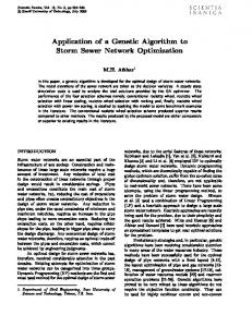
Two difficulties that often arise in the L P formulation of networks are the representation of the network in L P form and the complications that arise in using LP sensitivity analysis due to degeneracy. When these models are presented in network form, the following are essential and realistic assumptions: (a) The network is directed and acylic, i.e. there is no directed loop. Our algorithm detects successfully the existence of any cycle, and identifies the offender arcs which create such a hidden loop even outside of the optimal path. (b) Every node must be accessible from any other node, that is, there is no more than one network. (c) Every node, except possibly the origin and the destination nodes, is connected to at least two other nodes (there are no loose nodes). (d) The network does not contain parallel arcs (i.e., two or more arcs with same tail and head nodes. Violation of these assumptions is not legal but can occur due to common clerical errors. The following is an illustration. Consider the network shown in Fig. 1. The LP formulation for the C P (and SP) for this network is: Max (or Min) 5X,,

+ 8 X 2 , + 4X3, + 3Xs4 + 2X43


Figure 1 Separate network and/or cycle resulting from data entry error

subject to Downloaded by [University of Illinois at Urbana-Champaign] at 22:10 21 August 2013

XI, = 1

XI, X,, X,, X,,

- X2, = 0 - X,, = 0 - X43= 0 - X,, = 0

X,,

= 1.

The CP has an unbounded solution and the SP a unique solution. But both of these solutions are wrong, since both assumptions (b) and (c) are violated. Figure 1 makes these observations obvious. However, the LP formulation does not reveal this information easily. Similar difficulties arise in network-based algorithms, e.g. in finding the SP in a,network with negative length [46]. Further, it is very likely to have an optimal degenerate solution in network models. If one is not careful, LP sensitivity results obtained using available software may be misleading and incomplete. Whenever there is a degenerate optimal solution, depending on which redundant constraint is deleted, one gets a different final tableau which may result in a different set of sensitivity limits. Brute force could be used to delete one constraint at a time and then combine the results. However, it is possible to generate the other final tableaux from a given primal degenerate final tableau Table I Specialized network-based solution algorithms and their limitations ---

Problem

Most Popular Algorithm

Limitations -

AP

Hungarian

CP MF

Critical Path Method Ford-Fulkerson

SP

Dijkstra

TP

Stepping Stone

-

-

-

-

-

-

-

-

To "draw the m m m u m number of lmes to cover all the zeros In the reduced cost matr~x"may not be an easy task [71] and 1s h m ~ t e dto 2-d~mens~onal problems [95] May result in a non-critical path [15]. T o ensure termination arc capacities K E jmust be integervalued. Otherwise, may converge to an incorrect solution ~501. All C,, must be nonnegative [31]. Any arc with C,, = 0 must be removed. This restricts the sensitivity analysis for such arcs 11431. Among others, finding an initial basic feasible solution, and circuits in each iteration may not be easy [16].


219

and then perform the desired postoptimality analyses based on each tableau. Given a final tableau one first checks to find if there are multiple so1utions. If multiple solutions exist, then one generates all multiple solutions. Discard any that results in the same optimal strategy (basis changes but e.g, shortest-path, optimal assignment does not change). If any do result in a distinct optimal strategy then pick one. This process is depicted in Figure 2. An illustration of the process to handle PA optimal with degeneracy is given in the Appendix.


1.3 Solution Algorithms For Network Models

There are many specialized solution algorithms available for each of these problems [5,57,94,106,111,114]. These classical models have been dealt with in diverse fields such as network flows, combinatorial optimization, operations research graph theory and the literature is extensive. These different fields use different vocabulary to denote the same concepts and there is no standard notation. The most popular solution algorithms are listed in Table I, along with the major drawbacks of these algorithms.

d Final Optimal Tableau

Any multiple STRATEGIES

PICK ONE

Is optimal DEGENERATE

Perform the desired postoptimality analyses

I

Generate all other final tableaux

Perform the desired postoptimality analyses based on each tableaux Use UNION (for OSA, PSA) , and INTERSECTION (for others)

Figure 2 Postoptimality analysis of the multiple solution and/or degenerate cases.

220


Table I1 Obstacles in the existing primal and dual simplex solution algorithms Method Tabular simplex

Network simplex

Tabular dual simplex


Network dual simplex

Starting Conditions/Pivoting Operation Equality constraints not allowed, i.e. need artificial variables, penalty terms with large numbers which creates computational instability and round off errors [42,105]. Need artificial arcs with arbitrary large positive costs and capacities to obtain an initial spanning tree structure which may create computational instability and round off errors. [90]. Equality constraints not allowed, each equality constraint must be converted into two inequalities. Slack and surplus variables must be added which enlarge the tableaux and increase computational complexity [58,90]. Highly degenerate. Similar to the stepping stone solution algorithm, each iteration might need several &-perturbationswhich may create round off errors [66, 1511.

Notice that although these models are closely related to each other, there are fundamentally diferent strategies to exploit the special structure of each problem. Other solution methods (well over 100) are available (see the Reference list). The following is a very short list of other approaches: replacement of arcs, dynamic programming, matrix-based, analog approach, decomposition techniques, heuristic approach, and sorting technique. Although these algorithms provide new insights, they do not lend themselves toward a unified approach to an efficient strategy nor are they useful in PA. Since these problems can be formulated as linear programs, one expects the standard simplex method to be an attractive solution procedure. However, the simplex method does not exploit the underlying special structure of these models and cannot compete computationally with the faster specialized methods. The simplex-based network algorithms exploit the underlying network structures. However, the needed simplex operations are performed in the context of network flow with a specialized terminology. For example, in a network formulation, the simplex basic solution is the spanning tree, the pivoting operation is the movement from one spanning tree to another, variables are arcs, constraints are nodes, and the coefficient matrix is called the node-arc incidence matrix. Using network terminology, the network dual simplex algorithm satisfies the node balance constraints but might violate the arc flow capacities. By contrast, the network simplex satisfies the arc flow capacities and strives to balance the node constraints. The parametric network simplex algorithm is essentially similar to the dual network simplex except that it allows violation ofnode balance constraints at the source and the sink nodes [125]. These algorithms can work entirely with the network and no explicit tableaux are needed. The adaption of simplex methods to network optimization problems through a network provides unification of the various problems, but maintains all the inefficiencies of simplex. Even sensitivity analysis, long available in the simplex, has been only recently transferred to the network simplex methods. Table I1 outlines the major difficulties in both tabular and network-based classes of LP simplex and dual simplex solution algorithms. Computational studies have indicated that the network simplex algorithm is consistently superior to other network algorithms, see e.g., [7-9, 76, 80, 87, 1151. This has motivated us to have another look at the simplex approach. The proposed simplex


22 1

variant obtains an optimal solution from a good (warm-start) basic solution that may be either primal or dual infeasible. It builds on the strength of the self-dual simplex algorithm in that it can be initiated from any basic solution [56, 1501. This approach also facilitates PA since it easily handles the addition/deletion of arcs, side constraints, and more general perturbation. Partly because of these difficulties, the specialized network-based algorithms, such as those shown in Table I became the standard solution algorithms. However, their inability to handle the addition of simple constraints to the network is a major drawback. These so-called side constraints, such as capacitated conditions in T P [3,92], destroy the special structure of the network problem [32,51].


1.4 Strategy For New Simplex-Like Algorithm There are numerous distinguishing features of the LP formulation of these models. The coefficient matrices in all these models are totally unimodular [30,138] which simplifies the Gauss-Jordan pivoting operation [loo, 120, 1381. There is always an integer optimal solution whenever capacities, supplies, and demands are integer. There is no duality gap for these problems, therefore, the readily available solution to the dual problem would be the shadow prices which provide useful managerial information. These problems always have a basic feasible solution (never unbounded, never infeasible), as well as a redundant constraint. Finally, these models have a large number of equality constraints and certainly all equality constraints are active at the optimum solution. A recent stream of work [13-17, 21-24] has reexamined the simplex approach to these and other relevant problems by taking advantage of these special features. This paper provides a single unified algorithm for all five problems. Furthermore, this algorithm makes available the full power of simplex sensitivity analysis. More import-

r

SET UP Reliminary Phase (For Each Model AP. CP, MF, SP & TP)

AP, CP,MF,SP

I

1

I

PUSH

Basic Variable Set Augmentation Phase (Uses Simplex Rules)

Ophmal~tyPhase (Uses Simplex Rules)

TP

!

I Feasrbrliry Phase

AP,CP, SP

Final Simplex Tableau

More-For-Less Solut~on

Figure 3 General strategy for the proposed solution algorithm.


222

H.ARSHAM AND M. OBLAK

antly, it also facilitates perturbation analysis including structural changes in the nominal problem. The proposed simplex-like solution algorithm avoids artificial, surplus, and extra slack variables. Figure 3 provides an overview of the proposed general solution strategy. The algorithm consists of preliminaries for setting up the initialization followed by three main phases: Basic Variable Set Augmentation, Optimality, and Feasibility. The Basic Variable Set Augmentation Phase develops a basic variable set (BVS)which may or may not be feasible. Unlike simplex and dual simplex, our approach starts with an incomplete BVS initially and then variables are brought into the basis one by one. This strategy pushes towards an optimal solution. Since some solutions generated may be infeasible, the next step, if needed, pulls the solution back to feasibility. The Push-and-Pull strategy for general L P is developed in [17]. The Optimality Phase satisfies the optimality condition and the Feasibility Phase obtains a feasible and optimal basis. All phases use the Gauss-Jordan pivoting transformation used in the standard simplex and dual simplex algorithms. The proposed scheme is as follows: Step 1. SET UP: The initial tableau may be empty, partially empty, or contain a full basic variable set (BVS). Step 2. PUSH: Fill-up the BVS completely by pushing it toward the optimal vertex. Step 3. PUSH FURTHER: If the BVS is complete but the optimality condition is not satisfied, push further until this condition is satisfied (i.e, a primal simplex approach). Step 4. PULL: If the BVS is complete, and the optimality condition is satisfied but infeasible, pull back to the optimal vertex (i.e. a dual simplex approach). Not all of the network problems must go through the Set Up, Push, Push Further, and Pull sequence of steps. SP, and AP go through steps 1,2, and 4; C P goes through all steps; while M F goes through steps 1,2, and 3. Finally T P goes through steps 1 and 4 only. The T P is initiated with supply and demand parameters, while all other models are initiated without parametrization. The rationale for the sequence of steps and the distinct initialization of T P is provided in Section 2. In essence, this novel approach generates a tableau containing all the information we need to perform all parts of PA, as well as resolving the "more-for-less" phenomenon of TP. The large number of equality constraints with zero and one as their right-handside values (except possibly TP) raises concern for primal degeneracy [54, 55, 60, 66, 69, 1511. In the proposed solution algorithm, the B V S Augmentation Phase does not replace any BV's, and the Feasibility Phase uses the dual simplex rule, therefore, there is no degeneracy in these two phases. However, degeneracy (cycling) may occur in the Optimality Phase, which may be needed only for C P and M F models after the B V S Augmentation Phase is completed. This strategy reduces the possibility of any cycling. In the case of cycling in the Optimality Phase, this could be treated using the simple and effectiveanti-cycling rule for simplex method [37,53,70,86]. Out of the many problems solved by hand using our algorithm, we encountered no cycling. It is common in applications of these models to have side constraints in the nominal model. Network-based approaches to problems with side constraints are reported in [3,31,32,51] and extensive revisions of the original solution algorithms are required to handle even one side constraints. Additional difficulties arises from multiple side constraints [I 171. In the proposed algorithm, when the optimal solution without the



223

side constraints does not satisfy some or all of the side constraints, one can bring the "most" violated constraint into the final tableau by performing the "catch-up" operation [I, 191. After doing so, one can use the Feasibility Phase to generate the updated final tableau (and by introducing appropriate cutting planes if needed, to ensure the integrality of the solution). As part of PA we are also interested in any structural changes to the nominal network. To the best of our knowledge, there are only a few references [59,131] which deal with adding an arc to the network and furthermore, updating the optimal solution requires solving a large number of subproblems. The dual problem is used to determine whether the new arc changes the optimal strategy and if so, reoptimize the new network. We distinguish between basic and non-basic deleted arcs. If the deleted arc is a non-basic variable, the solution remains unchanged. However, if the deleted arc is a basic variable, the proposed algorithm replaces the deleted variable with a currently non-basic variable by using the optimality phase. Details are given in [I]. 1.5 Network Perturbation Analysis (PA)

Our primary concern is to design a solution algorithm useful to conducting perturbation analysis (PA). For the AP, CP, and S P we are concerned with the cost coefficients, i.e. objective function PA, while for M F the arc capacities, i.e. RHS values, are of concern. The PA of the T P is interested in both the RHS values and the cost coefficients i.e., PA of supplies/demands and the costs of the routes. We place a heavy emphasis on the various aspects of PA useful to the manager in the context of managing a variety of uncertainties in all phases of network management, namely, analysis (i.e. when the network exists), synthesis (i.e. when the network does not exist yet), and control (i.e. operational what-if questions), see e.g. [I, 29,35,99, 117, 126, 1441. Perturbation Analysis: As the name implies, PA deals with a collection of managerial questions related to so-called "what-if" problems in maintaining the current optimal strategy, i.e. preservation of the current optimal basis generated by the proposed solution algorithm. PA starts as soon as one obtains the optimal solution to a given nominal problem. There are strong motivations for performing PA. The network manager can use PA explicitly to: 0

0

0

0

0

help determine the responsiveness of the solution to changes or errors in controllable input values used in the model, test the responsiveness of model results to changes in uncontrollable inputs, and thereby offer valuable information for appraising the relative risk among alternative courses of action, adapt a model to a new environment with an adjustment in the parameters and validate the model, provide systematic guidelines for allocating scarce organizational resources to data collection and data refinement activities by using the sensitivity information, determine a parametric perturbed region in which the current strategic decision is still valid.

These needs can be served by one or more of the following results from various available L P types of PA for any of the models' cost parameters, capacity parameters, and supply/demand parameters:

224


General Perturbation Set: A set of ranges for which, given simultaneous changes from the nominal values in either direction (increase or decrease), the current optimal basis remains optimal. This provides the largest set of perturbations for costs, arc capacities, and supplies/demands. As long as all parameter values remain within the perturbed set, the current optimal basis is preserved. For the TP, the intersection of the perturbed cost set with the perturbed supply/demand set provides the largest set for simultaneous and independent changes of all costs, supplies, and demands.


Tolerance Analysis ( T A ) : Provides a range of simultaneous and independent percentage changes from the nominal values in either direction (increase or decrease) for each parameter while maintaining the current strategy. Individual Symmetric Tolerance Analysis ( I T A ) : Provides ranges for simultaneous and independent equal percentage change from the nominal values in both directions for each parameter, while maintaining the current strategy. This provides a range, e g , for each cost, with the nominal value at its center. Symmetric Tolerance Analysis ( S T A ) : Provides ranges for simultaneous and independent equal percentage change from the nominal values in both direction for all parameters while maintaining the current strategy. This provides ranges with equal half-length expressed as the percentage of the nominal values, e.g. for all costs. Parametric Sensitivity Analysis ( P S A ) : Provides the largest positive step size for which, simultaneous, but dependent changes in a given direction (i.e. dependency), maintains the current strategy. This provides the maximum magnitude of change, e.g. for dependent costs. PSA provides the largest (positive) step size for which changes along a given vector (scenario) preserves the optimal basis. We are not concerned with parametric programming for network models [150]. The 100% Rule: This provides suscient conditions for simultaneous and independent increase (or decrease) for all parameters. Ordinary Sensitivity Analysis ( O S A ) : Permissible change in any specific parameter while holding all other parameter values unchanged. For example, this provides a range for the change of any spec$c cost holding all other costs unchanged. More-for-less (nothing) Situation ( M F L )for T P : Find the maximum additional shipments and its distribution when the MFL condition exists in the optimal solution for TP.

1.6 Network-Based Approaches to P A

Although all aspects of PA have been developed [67] for general L P models, with the possible exception of dealing with optimal degeneracy, even ordinary sensitivity analysis is rarely performed on network optimization because the final solution generated by the existing specialized network algorithms does not contain enough information to perform sensitivity analysis. Application of a transformation scheme to attain the integrality condition for the nominal problem in the network-based algorithm makes PA complicated to interpret. A similar problem exists in treating the side



225

constraints using the Lagrangian relaxation method [3,4,31]. In network simplex, the basis matrix, B, is limited to the equality constraints (using the upper bound implicit approach), therefore the basis matrix, B, does not contain enough information to perform postoptimality analysis of the arc capacities in a maxflow problem [9]. It appears that research has been directed more toward the development of faster network solution algorithms, and has virtually ignored the PA, see e.g., [6,7,10,28,33,44, 68,78,89,108,110,135,139]. In dealing with data perturbation, the existing commercial software [I021 requires the brute-force approach of separate runs for different scenarios [34]. The very popular educational software LINDO [127], and the specialized T P programs in QSB [45] and NETSOLVE [88] are unable to perform OSA on supply/ demand for the TP. Unfortunately, these software are coded under the unnecessary and unrealistic assumption that there is no redundancy among the constraints, or that the perturbed T P must remain balanced. CPLEX [36,102], the current state-of-the-art code for solving network problems, incorporates nothing special for network sensitivity analysis. After the network optimizer is called, and if the given problem is a (pure) network, then a basis is produced that will be optimal. If the regular optimizer is run using this basis, then 0 iterations will be necessary to verify optimality, after which all the usual L P sensitivity analysis information is available. The problem is that even the LP ordinary sensitivity analysis is not well-adapted to network problems, particularly for supply/demand perturbations. There are a few references dealing with ordinary sensitivity analysis [59, 130, 132, 137, 1421 for networks, however, they require significant additional computation beyond the solution algorithm. Ravi and Wendell's [I181 use of symmetric tolerance analysis with a network solution algorithm is shown to be unnecessarily restricted in Section 3.3.5. The sensitivity analysis proposed in [41] is useful when the model contains a large number of common (equal) cost coefficient (or RHS) values however, at the expense of increasing the size of the problem to be solved. Two recent developments in network-based sensitivity analysis, namely the combinatorial approach [4], and the network-simplex approach [9,104], can only handle integer changes. The combinatorial approach requires the solution of a totally different new M F problem for each unit change in any cost coefficient, until infeasibility is reached. It requires a new S P problem for each unit change in capacity and each unit change in two supplies (one increase, and one decrease), or each unit change in two demands (one increase, and one decrease). The network simplex approach to sensitivity analysis can handle any number of unit changes, however, the pattern of change is also restricted to that used in the combinatorial approach (for more details see [4]). Neither of these two approaches produce any managerially useful prescriptive ranges for the sensitivity analysis. Additionally, a prerequisite for these approaches is to have the anticipated direction of changes. From the managerial point of view, anticipation of possible scenarios may not be an easy task. Numerous papers identify the MFL sitation, [47,48, 85, 124, 1321, and all use the stepping stone as the solution algorithm. Unfortunately, the question of how much additional shipment is optimal and how to distribute these extra units is left to trial and error. Use of the stepping stone algorithm to perform parametric sensitivity analysis is very tedious [62,132]. The parametric flow approach to sensitivity analysis [43,123] is also tedious. The PA of the T P proposed in [16] uses a symbolic supply-demand



226

version of a new simplex-type solution algorithm developed in [21], therefore, its computer implementation requires symbolic-based software [12,18] such as MAPLE. Furthermore, its treatment for finding the optimal additional shipments requires solving an associated larger linear program. The proposed PA in this paper is very efficient since it uses the same data and the same manipulations as the solution algorithm. The solution algorithm provides the necessary information to conduct all parts of PA including additional constraints or structural changes. Figure 4 provides various aspects of the PA. In cases where the optimal solution is not unique, one must be careful in using any part of the PA results, because the results may not be correct for the alternative optimal solutions, see e.g. [134]. This point is stressed in Figure 2. The development is straightforward and requires no reference to any theory of the general LP nor to the network-based algorithms for justification. The goals are theoretical-unification and extensions, as well as advancement in the practical implementation of network optimization with data perturbations. The remainder of this article is divided into four parts. Section 2 provides the new simplex solution algorithm which includes the MFL identification and solution for the

I

Final Simplex Tableau

I

AP,CP. SP

1

TP

MF

, TP I , I

Cost Perturbed Set

Capacity Perturbed Set

upply and Demand Pembed Set

Individual Symmetric

Symmeaic Tolerance Analysis

Scnsitiv~tyAnalysis

Sensitivity Analysis

Figure 4 Various aspects of the perturbation analysis.


22 7

TP. The optimal tableau provides the necessary information for performing various parts of the PA analysis. Section 3 establishes and demonstrates perturbation analysis for cost, capacity, and supply and demand respectively. Section 4 is devoted to some managerial implications and new directions for future research. In the Appendix, we walk through the different phases of the proposed solution algorithm and PA parts by solving one numerical example for each model.


2. THE SIMPLEX-LIKE NETWORK ALGORITHM This section describes the set up of the initial simplex-type tableau for the classic network models and a detailed description of the proposed algorithm. Our main theme is to formulate and design a solution algorithm with the capability of providing perturbation analysis. All these models have one redundant constraint. Eliminating any one constraint yields a non-redundant set. Rather than arbitrarily eliminate a constraint, the new algorithm eliminates the constraint which will most reduce the number of iterations at the BVS Augmentation Phase. General Notation: Gauss-Jordan Pivoting Basic Variable Basic Variable Set Feasibility Pivot Row (Row to be assigned to the variable coming in BVS) Pivot Column (Column associated with variable to come in BVS) Pivot Element Optimality Open Row. A row not yet assigned to a BV. Labelled (?). Label for a row which is not yet assigned a BV (Open Row) (?I RHS Right Hand Side C/R Column Ratio, RHS/PE GJP BV BVS FE PR PC PE OP OR

The algorithm consists of the preliminaries for initialization contained in Section 2.1 followed by three main phases. The BVS Augmentation Phase develops a BVS which may or may not be feasible. Unlike standard simplex and dual simplex, this variant allows for an incomplete BVS initially. Rows not associated with a BV are labelled with "?'and are considered "open". Initially, all or some rows are open. The Optimality, OP Phase, develops an optimal BVS. The Feasibility, FE Phase, obtains a feasible and optimal solution. All three phases use the GJP, however, they differ in the method used to select the pivot element, PE. The BV Augmentation Phase and O P Phase use Simplex criteria modified to select only open rows not already assigned to a BV and achieve optimality. This strategy pushes towards an optimal solution, and sometimes forces the solution into non-feasibility. The FE Phase, if needed, pulls the solution back to feasibility.


228

2.1


2.1.1

Preliminary Phase Assignment problem

Step 0.0-AP Cost Matrix Formulation 0.1 -Row-Column Reduction (or Column-Row Reduction) From each row subtract the smallest cost. Similarly, subtract the smallest cost in each column. 0.2-Eliminate Redundant Constraint Identify row or column with the most zeroes for reduced costs. Break any ties arbitrarily. Eliminate the corresponding constraint. 0.3-Set U p the Simplex Tableau Use a row for each constraint and a column for each variable. Do not add artificial variables. 0.4-Identify BVS For each column which is a unit vector, label the row containing the "one" with the name of the variable for the column. Label the remaining rows with question mark (?). 0.5-Delete BV Columns and the Start B V S Augmentation Phase. 2.1.2

Critical path problem

Step 0.1 -Identify Redundant Constraint Identify the variable X i j with largest C i j in the objective function. Break any ties arbitrarily. Identify the two constraints containing the variable. Eliminate the constraint with smallest RHS (break any ties arbitrarily). Set up the initial simplex tableau without adding any artificial variables and then start BVS Augmentation Phase. 2.1.3 M a x Pow problem An efficient way to handle the upper bound constraints (i.e., the capacity constraints) is to use the bounded variable simplex method [104]. However, we treat them like equality constraints after adding slack variables. By doing so, we will be able to perform PA on the arc capacities. For M F with positive lower bounds on all or some arc flows, we will relax them first and then, after obtaining the final simplex tableau, we bring in the violated ones in the final tableau using the dual simplex pivoting rule as needed. Clearly, an alternative approach for such problems is to substitute gij + Lij for any f i j with lower bound Lijon its flow. However, we recommend the first approach since the latter may complicate the interpretation of the PA for Lij. Step 0.1 Standard M F Form Convert the L P formulation into the standard form of M F as follows: a) The objective function is the left hand side of first constraint. b) Drop the 1st constraint and the last constraints from the set of constraints. c) Add slack variables for the set of inequality constraints except the non-negativity constraints. D o not add artificial variables. Step 0.2 Simplex Initial Tableau Use a row for each constraint in the standard form of MF. Use a column for each variable except the slack variables.


229

Identify BVS: The first few rows belong to the equality constraints with a question mark (?) and the remaining rows with the slack variables. The last row is the Cij row containing the coefficients of the objective function. Start the BVS Augmentation Phase. 2.1.4 Shortest path problem Step 0.1 Elimination of the Redundant Constraint Identify the X i j with smallest C i j in the objective function. Break any ties arbitrarily. Identify the two constraints containing that variable. Eliminate the constraint with smallest RHS (break any ties arbitrarily). Set up the initial simplex tableau without adding any artificial variables and then start BVS Augmentation Phase.


2.1.5

Transportation problem

0.1 Set U p the Initial Tableau for Parametric T P Relax non-negativity constraints. Multiply each equality constraint by ( - I), use ri, k j as basic variables. Use one row for each constraint and a column for each X i j variable, then start PULL phase to find solution. 2.2 Basic Variable Set Augmentation Phase 1.0 Iteration Termination Test I F (?) Label exists, there are Open Rows. THEN continue the BV Iteration. OTHERWISE BVS is complete, start PUSH FURTHER Phase for CP, M F models. Start PULL phase for AP, SP models. 1.I BV Selection of PE PC: Select the Largest C i j(the smallest for min problems) and any ties are candidate column(s). PR: Select OPEN ROWS as candidate rows. PE: Select the candidate row and column with the smallest non-negative C/R. Break ties by selecting the variable X i j with the smallest i. Further tie breaker: select X i j with the smallest j. If no non-negative C/R, choose the C/R with the smallest absolute value. If the pivot element is zero, select the next best Cij. 1.2 Augmentation a) Perform GJP. b) Replace the (?) row label with the variable name. c) Remove PC from the Tableau. Continue BVS Iteration (Loop back to 1.0)

2.3

Optimality Phase 2.0 Optimality Iteration Termination Test I F any C i j is positive (negative for min problem) THEN continue the O P


230


Iteration, OTHERWISE O P is complete, start PULL Phase for CP. Stop for MF. 2.1 BV Selection of PE PC: Select the Largest Cij (the smallest for min problem) and any ties as candidate column(s). PR: Select the candidate row and column with the largest positive C/R. If no positive C/R choose the C/R with the smallest absolute value. If the pivot element is zero, select the next best Cij. 2.2 BVS Iteration a) Save P C outside the tableau. b) Perform GJP. c) Exchange P C and PR labels. d) Replace the new P C with old P C with all elements multiplied by ( - 1) except the PE. Continue OP Phase (Loop back to 2.0) 2.4

Feasibility Phase FE Iteration Termination Test I F RHS is non-negative THEN Tableau is Optimal for AP, CP, and SP, Go to MFL Phase for the TP. OTHERWISE continue FE Iteration (Step 3.1). FE Selection of PE PR: row with the most negative RHS. Break ties by selecting the variable X i j with the smallest i. Further tie breaker: select X i j with the smallest j. PC: column with a negative element in the PR. Tie Breaker: column with the smallest Cij. Further Tie Breaker: Cij with largest i. Further tie breaker: C i j with the largest j. FE Transformation a) Save P C outside the tableau. b) Perform usual GJP. c) Exchange P C and PR Labels. d) Replace the new P C with old P C saved in (a). Continue FE Iteration (Loop back to 3.0)

2.5

M F L IdentiJication and Solution for T P 4.0 Removal Termination Test I F no ri and/or k j with negative RHS in basis THEN Go to step 4.3 OTHERWISE continue Iteration (Step 4.1) 4.1 Use dual simplex pivot selection 4.2 Perform shortcut G J P operation Continue REMOVAL (Loop back to 4.0).



23 1

M F L Existence Identification and Solution If there is any ri or k j variables with positive (zero) RHS, we have M F L (nothing) situation. Find the MFL solution and its distribution. G o to step 6 Solution to the nominal T P Problem Remove ri and k j Variablesfrom basis Removal Termination Test If no ri and no k j vaiables with positive RHS, Then tableau is optimal for the nominal TP. Construct the B-inverse (which is the columns of these parameters) for postoptimality analysis. OTHERWISE, Multiply rows with positive ri and/or k j by (- 1). Use dual simplex pivot selection Perform shortcut G J P operation Continue REMOVAL (Loop back to 4.4). DUAL SIMPLEX PIVOT SELECTION PR: row with the most negative RHS. Tie Breakerxelect variable ri. Further tie breaker: select ri with the smallest index i. PC: column with a negative element in the PR. Tie Breaker: column with the smallest Cij.Further ties: select Cijwith the smallest i. Further tie breaker: select C i jwith the smallest j. SHORTCUT GJP OPERATION a) Save P C outside the tableau. b) Perform usual GJP. c) Exchange PC and PR Labels. d) Replace the new P C with old P C saved in (a). e) I F step 4.6 multiply this P C by ( - 1) E N D OF SOLUTION A L G O R I T H M 2.6

Outline Proof of Algorithm

The algorithm consists of a preliminary step to generate an initial tableau for each model followed by three main phases. The first is the B V S Augmentation Phase to develop a basic solution which may or may not be feasible. The second is the OP Phase to generate a BVS which satisfies optimality (i.e. optimality condition). The third is the FE Phase to obtain a feasible optimal solution. All three phases use the GJP, however, they differ in the method used to select the PE. The B V S Augmentation Phase uses simplex criteria modified to enter one variable at a time into an open row while moving toward a vertex which is "close" to the optimal vertex. This strategy pushes towards the optimal solution, which may result in falling short of optimality or pushing too far into nonfeasibility. The OP Phase, if needed, pushes further toward optimality (may push too far into nonfeasibility). The FE Phase, if needed, pulls to a feasible solution which is optimal. The concise statement of the proposed scheme is as follows:


232

Step 0 Set Up: Start with the initial tableau with empty, partially full, or full basic variable set (BVS). Step 1 Push: Fills-up the BVS completely while pushing toward the optimal vertex. Step 2 Push Further: If the Optimality condition is not satisfied, push further until the optimality condition is satisfied (i.e. a primal simplex approach).


Step 3 Pull: If the feasibility condition is not satisfied, pull back to the optimal vertex (i.e. a dual simplex approach). The solution for all models starts with step 0. The T P initial tableau is set-up with supply and demand parameters, while all other models are not parameterized. Not all these problems must go through the Push, Push Further, and Pull sequence of steps. SP and AP go through steps 1 and 3; C P goes through all steps; M F goes through PUSH and PUSH FURTHER. Finally T P goes through only PULL since it is set-up with a complete BVS with optimality condition satisfied. The rationale for these distinct set of steps is given in Table 111. Optimality is attained when all Cij 6 0 for max problems (Cij2 0 for min problems). The algorithm starts with all Cij2 0. We show that the operations we use to obtain a basic and feasible solution results in Cij< 0. In the BV Augmentation Phase the selection criteria leaves one possibility, selection of the largest Cij. This may cause some Ci;s to become non-positive after pivoting. If pivoting is not possible (no finite CIR) we select the next largest Cij. However, the value of the largest Cijis unchanged since the pivot row element in its column is zero. By this pivoting selection rule the proposed algorithm is free from degeneracy which may cause cycling. The other remaining two phases are the ordinary simplex and dual simplex where for convenience we use the reduced pivoting rule. The reduced pivoting rule produces the same tableau as the usual pivoting. Knowing these problems are never unbounded and never infeasible, we must show that the proposed algorithm converges successfully. To prove this is suffices to show each phase terminates successfully, since the path through the phases of the algorithm (see Figure 3) does not contain any loops. The Set Up phases use the structure of the models to fill-up the BVS as much as possible requiring no G J P iterations. The Push phase completes the BVS using

Table111 Rationale for sequence of steps for each problem, where: P = BVS partially completed, C = complete BVS., U = condition unsatisfied, S = condition satisfied, D = don't care, N A = not applicable Set Up

Problem AP (min) CP(Max) M F (max) SP (min) T P (min)

Push

Push Further

Pull

Feas.

Opt.

Feas.

Opt. Feas.

NA S S NA NA

NA D

S

S NA NA

NA

BVS

Opt.

Feas.

BVS

Opt.

P P P P C

S

D

U

D

D

S

U

C C C C NA

S

S

S S S S

S D NA

U

U

S NA

S S S

S S NA S S


233

ordinary simplex rules. The number of iterations is finite since the size of the BVS is finite. This phase is free from degeneracy (which may cause cycling) since variables are only entering (none departing). For this reason, deletion of basic columns is also permissible, which reduces the complexity significantly. At the end of the Set Up and Push phases we have a basic solution. The Push Further and Pull Phases terminate successfully by the well-known theory of simplex and dual simplex respectively.


2.7 Computer Implementation Issues

The description given up to now of our proposed algorithm aimed at clarifying the underlying strategy and concepts. A second important aspect that is now considered is efficient computer implementation. Practical networks may have hundreds or thousands of constraints and even many more variables, e.g. a T P with m origins and n destinations has m + n - 1 constraints and m e n variables. Network models also have a large percentage of zero elements in the coefficient matrix (i.e. a sparse matrix). Our proposed simplex-like method as described is not efficient for computer solution of large-scale problems, since it updates all the elements of the tableau at each iteration. Some useful modifications of the proposed algorithm as well as its efficient implementation will reduce the number of computations and the amount of computer memory needed. This section describes how an efficient implementation of the solution algorithm capable of solving large-scale problems [52, 93, 100, 103, 1291 could be developed. Adaptation of sparse technology is motivated from the fact that for the large sparse problem, an iteration of the revised simplex method takes less time than a iteration of the standard simplex. Many researchers [26,27, 841 and references therein found that the primal simplex algorithm is superior (i.e. faster, requires less storage) to others, including the out-of-kilter algorithm. Our implementation is a straightforward adaptation of our proposed simplex-like algorithm through appropriate use of data structure, e.g. [73, 1361, sparse technology [61], pivot strategy rules [52], [82], [83], as well as, triangularity of the constraint coefficient matrix [4]. Computer implementation of all phases of the algorithm is discussed. We are concerned with computational efficiency, storage, accuracy, we well as ease of data entry. 2.7.1

Sparsity and data structure

The density of a matrix is the ratio of the number of non-zero entries in the matrix to the total number of entries in the matrix. A matrix that has a low density is said to be sparse. The sparse matrix technology [113], is based on the following principles: only non-zero elements are stored, it attempts to perform only those computations which lead to changes, 0 the number of fill-in elements (i.e. non-zero) is kept small, any unused locations (zero elements) can be used for storing of fill-ins (non-zeroes produced later).



234

Sparsity technology enables us to reduce the total amount of work that is done in each iteration. A variety of schemes are available to avoid storing the zero entries of matrices. Since our calculations operate on tableaux by columns, we will discuss a storage structure, called a linked list, that makes it easy to access data by columns. A piece of computer memory must contain three entries: one to hold an entry from the tableau, one to hold a row number, and one for the pointer to hold the next memory address of the appropriate columns (see Appendix for an illustration). Having a matrix generator program in order to automatically generate constraints and the objective function, see e.g. [24], one can store the non-zero values in link list form. This scheme has minimal storage requirements and at the same time it has proved to be very convenient for several important operations in our solution algorithm and PA analysis such as permutation, addition, and multiplication of sparse matrices. For example, it can be shown that if b is a (1 by m) matrix and B is an (m by n) matrix that is stored as a linked list, then bB can be evaluated in d.m.n multiplication, where d is the density of B. An advanced variant of thls scheme is Sherman's compression, see e.g. [I 131 which is useful in storing triangularized matrices. Such an approach can be applied in all phases of our solution algorithm, as well as, for the needed matrix manipulations in our perturbation analysis. 2.7.2

The push phase

For the Push Phase one can construct a lower (block) triangular matrix by permuting matrix A with any row operation. Permute the columns with non-zeros in row 1 to the left; follow with columns having a zero in row 1 and non-zeros in row 2; then columns having zeros in rows 1 and 2 and non-zeros in row 3; and so on. When column k enters the basis, the updating procedure moves columns (k + I), (k + 2), . . . ,(m)all one place to the left and appends the incoming column at the extreme right to give a new matrix A,,,. The results remain a lower triangular in the subsequent row operations except possibly for the fill-in which is confined to the diagonal block only. An alternative approach is block triangular diagonalization to reorder to preserve sparsity (for details see Duff et al. [61] Sections 8.8 and 8.9).This approach is attractive since G J P operation maintains sparsity. In other words, this triangular structure is invariant under row or column interchanges to achieve sparsity within each block. A preliminary study exploiting sparsity in the T P model using Gaussian elimination for the primal simplex is reported by Brameller [39]. This approach could also be applied to our PUSH Phase. Employing the strategy of avoiding use of artificial variables, the PUSH Phase does not have a basis matrix at all. In the PUSH Phase, we start the initial tableau with a partially filled basic variable set (except for T P which is filled up), therefore the basic variable set is being developed. This particular crashing technique pushes toward a "vertex close to the optimal". One could use artificial variables as in revised simplex and proceed to other phases. Most professional codes incorporate some form of crashing techniques to provide the initial basis. Freund [65], and Bixby [36] start from an infeasible point. Pan [I091 starts from a "good" basis and does not introduce any artificial variables. Other starting procedures may be found in [82,110].


235


2.7.3 The push further and pull phases

Using the basis matrix B (now easy to construct using the initial tableau), any iteration in these two phases consists of the direction ofmovement (say k) by solving WB = C, in the Push Further Phase, and updating the pivot column y, by solving By, = a,, and finding the value of the new basic solution by solving Bx, = b. This basic solution is used in PULL Phase to find which current basic variable must leave the basic variable set (if needed), performing the row (or column) ratio test, and moving to the new basic solution by performing the pivot operation (i.e. updating the Bmatrix). In the computer implementation the inverse of the basis matrix is not needed. If B is a triangular matrix, then the foregoing systems of equations can be solved easily by a forward and two backward substitutions respectively. As in the revised simplex the inverse basis matrix B is not computed, instead, the basis is factored into elementary product form. Let B = E l . . . .E,, where each E, is an "elementary" matrix, that is, it differs from the identity matrix in exactly one column, which is the pivot column. We can also achieve efficiency in performing G J P operations in these phases from another point of view known as B = LU factorization of B, see e.g. Reid [119]. Matrices L and U are a lower and upper triangular matrices for which their inverse can be computed easily and the solving of the above systems of equations by inversion. In this approach L-' is stored as a sequence of "elementary" matrices and U is stored as a permuted upper triangular matrix. The Reid implementation of Bartles-Golub updating has a clever row exchange and column exchange preprocessing scheme that produces a triangular matrix for network models without the need for any eliminations. To update the B-inverse (i.e. re-inversion) for each G J P operation there are several ways, depending upon how the columns of new basis are arranged and what pivoting strategy is used [52]. Forrest and Tomlin [64] proposed an ingenious variant of the Bartles-Golub triangular factored updating procedure to exploit sparsity. This approach could lead to a decrease in accuracy through the introduction of round-off error. However, since we are working with integers (not real numbers) and not using any large numbers such as big-M, our computations are precise and reliable. A set of complete algorithms coded in Fortran 77 for these operations can be found in [61]. The approaches presented here can also be used in the PULL Phase which (as is) uses the usual dual simplex rules. Working with the triangularized of B rather than B itself has been shown to reduce significantly the growth of new non-zero elements (in particular for the generalized network), see e.g. [77, 971. It is well known that the basis matrix B is reducible to a unique triangular structure in our models. The very structure of the basis in these models allows for rearranging it to a lower triangular form. The fill-in is zero when the basis is triangularized. The general idea is to permute the rows and columns of the basis to make the rearranged matrix lower triangular. There are two phases namely front and rear phases. Front Phase: Among unassigned rows, find one with min count (no. of non-zeroes). If this count is 1, assign the row and its (only) unassigned column to the front and repeat; otherwise, exit. Rear Phase: Among unassigned columns, find one with min count. If this count is 1, assign the column and its (only) unassigned row to the rear and repeat; otherwise, exit.


Row 1 Row 2 Row 3 Row 4

Col. 1

2

3

x x

x

x x x

x

4

Count

x

3 1 1 3

Figure 5 Initial Pow and Column Counts.


Col. 1 Row 2 Row 3 Row 4 Row 1

2

3

x x x

x

4

x x x

x

Figure 6 Result of the Triangularization.

An illustrative Example: Figure 5, shows the initial matrix for an illustrative example. The count is the number of non-zeroes in rows/columns. Upon entering Front phase we find row 2 is a singleton, so it is assigned to the front with column 1. Then, row 3 is assigned to the (new) front with column 3. Next the Rear phase is entered, and the column singleton Col. 2 is assigned to the rear with Row 1. The result is shown in Figure 6. 2.7.4 Other pivoting and anti-cycling strategies

The simplex method in general is very sensitive to pivot selection strategy [37]. Goldfarb and Reid [81] provide a practical approach for steepest-edge pivoting. This rule, also referred to as the largest-increase rule, is to choose the candidate whose entrance into the basis brings about the largest increase (maximization) in the objective function. This usually reduces the number of iterations, however, it may increase total computing time (see also [147]). A large fraction of the time needed to perform an iteration can be spent in retrieving the data. For computer implementation the pricing components can be computed individually which allows for partial pricing and even multiple pricing strategies. This approach is best suited to our algorithm given the sparsity of our models. The impact of different choice rules with respect to practical efficiency is given in [9]. While degeneracy is not a problem in network-based algorithms such as FordFulkerson, it is a frequent phenomena in the network-based simplex algorithm [86]. Cycling is impossible to occur in our PUSH Phase, however, to prevent its rare occurrence in the PUSH FURTHER Phase the simple and effective Bland rule is suggested. Klafszky and Terlaky [91] successfully use Bland's pivoting rule to avoid cycling in the assignment problem. Other potential rules are also available. Other various network-based anti-cycling rules are given in [54, 55, 69,70, 79, 981. Our discussion has been general. Clearly, for special cases e.g. in T P with m 0). Clearly, the vector {Ci;, Cif , CIJ

CgB can be written as: C,: = [- C,, C,,]. [ B - ' . N I IIT, where I is an identity matrix of order k, k is the number of non-basic variables in the final tableau, and T means transpose. Let (C$B)jbe the jth element in the reduced-cost vector (i.e, the last row in the final table). Let A = [ B - N / I I T ,and Tj = C . /Aj/ where I AjI is the absolute value of the jth column of A and C is the nominal cost coefficient vector, 1 < j < k. The cost coefficients in vector C are ordered as the basic variables appeared in the final table. From now on, we must differentiate between the cost coefficients associated with the basic variables and those with the nonbasic variables. a) Tolerance limits for cost coefficient of the basic variables For any cost coefficient of basic variable X,,, i.e., for c,,, the upper tolerance limit for C:, is: C:

= min{C,k[(C;B)j/Tj], and the upper limit form OSA},

where the min is over all j such that the element in the C:, row and the jth column of A is positive. The lower tolerance limit for C;, is: C:;

=~~X{C,,[(C;~)~ Tj], /-

and the lower limit from OSA}

240

-


where the maxis over allj such that the element in the C:, row and the jth column of A is negative. By definition 010 0. b) Tolerance limits for cost coefficients of the nonbasic variables For any cost coefficient of the nonbasic variable X,,, i.e., for c,,, the upper limit is and its lower limit for C;, is:

+ co,


- Tj], and the lower limit from OSA), C;; = rna~{C,,[(C,*,)~/

where the max is over all j such that the element in the (C:, row and the jth column) of A is positive. By definition 010 = 0. The symmetric tolerance limits reflect the maximum allowable equal percentage changes in both directions that holds simultaneously over all cost coefficients. The symmetric tolerance range is a subset of the tolerance limits, i.e.: Upper Limit = - Lower Limit = min[Cif, - Ci;, in % I over all i j Note that if the nominal SP is dual degenerate, i.e., one of (C*,,)j is zero, or whenever the nominal cost coefficient is zero, then at least one of the tolerance limits is zero. Occurrence of such a situation has a major impact on the symmetric tolerance analysis, making both upper and lower limits equal to zero for all cost coefficients. 3.2 Arc Capacity Perturbation Analysis

To address PA of the arc capacities simultaneously, we consider the following perturbed capacity M F problem: Max f subject to:

3.2.1

General perturbed set

The optimal solution to the above perturbed problem can be found from the final tableau of the nominal problem by the following argument: The G J P rijelements would be exactly similar to the slack variables Sijin the nominal problem, therefore it suffices to reconstruct the final tableau by deleting any column of f i j and adding new column vectors for basic variable Sij. We refer to this as the parametric final tableau. Therefore, the parametric M F solution has elements rij with the same coefficients as of Sij in the parametric final tableau. The body of the parametric final tableau is denoted by matrix B - ',vector b(rij)is the last column is this table which is B - [kij rij] where [kij + rij] is the parametric capacity column vector with kij rijas its ith row element as shown in Table V.

+

+


Table V. Parametric MF final tableau BVS

XB

Sij B-'

RHS Wij)


Our PA begins as soon as we get the parametric final tableau. The optimal parametric solution is a set of ( m+ n - 2) variables in the final tableau, whose values are denoted by the RHS column vector. The perturbed set is the largest set for which the current basis remains optimal:

R = {rij(b(rij)2 0, and rij 2 - kij}, where b(rij) = B-'.b + B- l.[rij] and [rij] is a column vector with rijas its ith element. Note that set R is non-empty since it contains the origin (rij = 0, for all i and j). Also set R is a convex set with linear boundary functions, by the virtue of GJP operations. It is a cone with the vertex at rij = - kij. This set could be used to check whether a given perturbed arc capacity has the same optimal basis as the nominal problem, and if so, to update the optimal solution for any perturbation from their original estimates. 3.2.2 Parametric sensitivity analysis Define a perturbation vector R specifying a perturbed direction of the arc capacities. Components of R are ordered as the basic variables appeared in the final tableau. As long as the parametric RHS vector is non-negative, the current optimal basis remains optimal. In other words, the problem is to find the largest 6 2 0 such that [B - 11.(b + 6R) 2 0, where 0 is a zero column vector with appropriate dimension. Define b' = [B-'1.R. Let S = {all basic variables for which the corresponded element in b' is 0, where 010 = 0 by definition. The lower tolerance limit for r, is: r; = max{b; [RHS*/ - Ti], and the lower limit from the OSA}, the max is over all i's such that (B-l), < 0. A similar procedure holds for k,. Notice that this calculation must be performed repeatedly using all basis inverse matrices. Clearly, the tolerance limits are the largest (m + n - 1)lower and the smallest (m n - 1) upper limits found for each parameter. The symmetric tolerance limits can be found as follows:

+

Upper Limit = - Lower Limit = min[min(r:,r:, . . . ,r:, k:, k z , . . , ,k:),

-max(r;,r;,

. . . ,r;, k ; , kz-, . . . ,kn-),in %I.

The symmetric tolerance analysis (STA) has been developed by Ravi and Wendell [I181 under non-degeneracy (primal and dual) assumptions. It provides no meaningful range for any cost coefficient if the final tableau of the nominal problem is either dual degenerate, i.e., whenever any element in the last row of the final tableau is zero (this is necessarily the case whenever there is an alternative solution), or any nominal arc cost value is zero. In such cases, the allowable change is zero for all cost coefficients. This obviously limits its application. Moreover, the STA can severely shorten its interval, especially when the network has many arcs. That is, as the number of arcs in the network becomes larger, the allowable change for STA can be expected to become smaller and smaller. Similar shortcomings exist for the STA of the capacities, and supply and demand parameters.

4. MANAGERIAL IMPLICATIONS AND CONCLUDING REMARKS In this paper we have focused on the following five prototype network models: Assignment Problem (AP), Critical Path Problem (CP), Maximum Flow Problem


246


(MF),Shortest Path Problem (SP), and Transportation Problem (TP).The first section included a short review of widely known network-based solution algorithms and demonstrates that all specialized algorithms which exploit special structure, while efficient, do not lend themselves easily to sensitivity analysis. The current approach is a variant of the self-dual simplex algorithm with warm start to bring a unified solution algorithm which is general, iterative, converging, finite, and theoretically attractive. The proposed method is computationally practical and stable since it avoids using artificial variables with big-M penalty terms (needed in the simplex method), and the artificial constraint with big-M on its right hand side (may be needed in the dual simplex, see e.g. [30]). In the proposed solution algorithm the working tableaux are simpler since the G J P operations are performed directly on Cijand not on the so-called reduced costs (an additional row). The algorithm is concise to state, intuitive, and easy to implement, since the only operation used is the G J P operation. In our discussion on computer implementation issues we pointed out that if the sparseness of these models is taken into account, it is possible to improve significantly the performance of the algorithm, for example by using the link list instead of a matrix generator. This presentation reflects the new developments in Perturbation Analysis (PA) which deal with a collection of managerial questions in the context of what-if analysis and data uncertainty. We place a heavy emphasis on designing a solution algorithm useful for PA. The proposed solution algorithm deals effectively with change and chance, and is compatible with other solution algorithms. In contrast to ordinary sensitivity analysis, the PA provides useful information related to ranges on simultaneous, dependent, or independent departures from the estimates and the impacts of such departures on the current optimal strategy (i.e, optimal basis). We developed PA for all parameters in these problems, the cost coefficients in the SP, AP, CP, and the capacities in the M F model. For T P we provide PA for cost and supply/demand as well as the more-for-less identification and solution. Although ordinary sensitivity analysis has long been available for linear programs (LP), solving the network problems with the standard primal and dual simplex is inefficient. Therefore, special network-based algorithms became the standard solution algorithms. However, they do not provide the information needed for conducting various parts of the PA as outlined in Figure 4. To overcome both difficulties, a new simplex-type solution algorithm is presented which is general, stable, compatible, and provides results which allows PA to be implemented on a spreadsheet. The final solution tableau provides the information required to handle any special cases, for example, a network with linear side constraints such as capacitated TP as well as other structural changes. If we are interested in finding all alternative optimal strategies, the last row in the final simplex tableau provides the necessary information. For example, if any non-basic Cij= 0, then there may be at least one alternative optimal solution. By bringing any variable with Cij= 0 into the basis one may generate a new optimal solution. Finding all alternative solutions is necessary since the results of PA for the current optimal basis may not be correct for others (see Figure 2). As was noted earlier, a curious property is associated with the TP, called the more-for-less (MFL) phenomenon. A managerial explanation for this phenomenon is



247

as follows: We say a given T P is "perfect" if the optimal solution has the least number of non-zero X i j among all TP's which have the same dimensions (i.e, number of origins and number of destinations). In the early development stage of any distribution planning system the T P could be almost perfect (simply by building plants where the markets are). If implemented over a period of time, the changes in demand and supply and/or unit shipment costs make the problem less "perfect". Note that in the M F L situation, the number of arcs in the optimal shipment route is always less, at least by one, when compared with the optimal strategy for the nominal TP. In certain cases, by supplying just enough more units, the new T P becomes closer to a perfect match. The MFL analysis could be useful in decisions such as increasing warehouse stocking level or capacity. In turn this could prompt a decision for advertising efforts to increase demand at the local market. Note that if an MFL situation exists, one must also consider other managerial issues, such as whether the additional holding cost balances against this saving, or the possibility of losing alternative opportunities. Notice also that the proposed M F L solution approach presented here is an algorithmic approach having the advantage of distributing the additional shipments, if any, in a systematic way rather than a trial and error approach, as in the stepping stone solution algorithm based methods. It also has advantages compared with the proposed method in [16] which requires solving an associated large L P problem. Unlike the existing network-based sensitivity analysis, our proposed PA provides several prescriptive uncertainty ranges. As long as the estimated parameters remain within ranges specified by the PA, the current optimal strategy remains optimal. From the managerial point of view, the PA results provide an assessment and analysis of the stability of the optimal strategy by monitoring the admissible range that preserves the optimal strategy. This permits evaluation of the impact of uncertainty in the data. PA also provides disclosure of the useful PA limits on simultaneous, dependent, or independent departures from the estimates and the impacts of such departures on the current optimal strategy. PA allows the manager more leverage in allocating scarce resources. Monitoring the admissible range of PA that preserves the current optimal strategy aids in determining how resources should be applied. Information about departure from these limits allows the manager to anticipate the consequences and to pre-determine back-up strategies. By using the PA results the network manager is now provided with means for discussion and analysis by the team members as to how to consider modifying the structure of the network prior to its implementation. The manager can anticipate a range of changes due to uncertainty or other reasons before a new strategy becomes optimal [126]. Using the critical path problem as a specific example, Winston [I431 stated correctly that: "The assumption that the critical path found by the critical path method will always be the critical path for the project network may not be justified." For example if an activity A was signijicantly delayed and an activity B was completed ahead of schedule, then the critical path might be different. The main managerial question is how much delay and how much ahead of schedule? Unfortunately, the answer is not generally given. However, we obtain this needed information using PA results (see Appendix for illustration). Notice that throughout the PA analysis we have assumed that the capacity, supply, demand and other input data such as costs are continuous. As a result, whenever some

248



data is required to be discrete (as in network-based approaches), we must add this admissibility condition to all parts of PA. Tolerance analysis introduced by Ravi and Wendell [I 181 is limited to finding symmetric tolerance limits, whereas we developed the general perturbation analysis from which tolerance analysis is apparent. The tolerance analysis given in [140,141,145] for general L P models are complicated. The proposed approaches in this paper have the advantage of being computationally practical, easy for the manager to understand and use, and provide useful information in all cases. As always, one must be careful when rounding the PA limits. The upper limit and lower limit must be rounded down and up respectively. This point, unfortunately is overlooked in both [140, and 1451. The optimal solution and the prescriptive PA results should serve as an aid to, rather than a substitute for, management judgement. Therefore, the network manager's experience must be incorporated in our proposed modelling results. We suggest the following directions for future research: -Efficient computer implementation for a comparative study [60,103], computational testing [26,28,37] and design of an intelligent computer-assisted system for data collection, modeling, and solution interpretation useful to the network manager. -Extend the algorithm to other combinatorial problems [I461 and networks with fractional linear objective functions, such as link utilization [20, 35, 101, 1161. The MFL analysis presented here might be extended to the general LP problem with equality constraints [22]. -Look into possible further refinement and then translate the proposed algorithmic strategy into specialized network version to make use of available technological advances of network-based optimization [149]. Pseudo codes version of all the processes presented in this study are available from the first author upon request. Acknowledgements We are most appreciative of the comments from the reviewers and useful information from Dr. Robert Bixby. Parts of this work are supported by The Commission on Office Laboratory Accreditation, Silver Spring, MD.

References [I] Adlakha, V. and Arsham, H. (1994) A warm-start dual simplex algorithm for the min flow in planar networks useful for postoptimality analyses, Submitted for publication [2] Adlakha, V., Gladysz, B. and Kamburowski, J. (1991) Minimum flow in (s,t) planar networks, Networks, 21,767-773 [3] Aggarwal, V. (1985) A Lagrangian-relaxation method for the constrained assignment problem, Computers & Operations Research, 12,97-106 [4] Ahuja, R., Magnanti, T. and Orlin, J. (1993) Network Flows: Theory, Algorithms, and Applications, Prentice-Hall, Engelwood Cliffs, New Jersey [5] Ahuja, R., Magnanti, T. and Orlin, J. (1991) Some recent advances in network flows, S I A M Reaiew, 33, 175-219 [6] Ahuja, R., Mehlhorn, K., Orlin, J. and Tarjan R. (1990) Faster algorithms for the shortest path Problem, Journal of A C M , 37,213-223 [7] Ahuja, R, and Orlin J. (1991) A fast and simple algorithm for the maximum flow problem. Operations Research. 37, 748-759 [8] Ahuja, R. and Orlin, J. (1992) The scaling network simplex algorithm, Operations Research, 40, Supplement 1, S5-S13 [ 9 ] Ali, A., Allen, P., Barr, R. and Kennington, J. (1986) Reoptimization procedures for bounded variable primal simplex network algorithms, European Journal of Operational Research, 23,256-263



249

[lo] Ali, A,, Padman, R. and Thiagarajan, R. (1989)Dual algorithms for pure network problem, Operations Research, 37, 159- 171 [ l l ] Anderson, D., Sweeny, D. and Williams, T. (1994) An Introduction to Management Science, West Publishing Co, St. Paul, MA [12] Arsham, H. (1994) The Gauss-Jordan matrix inversion is not optimal: A symbolic adaptation, In the Proceedings of the Fifth S I A M Conf on Applied Linear Algebra, 528-532 [13] Arsham, H. (1994) A solution algorithm with sensitivity analysis for optimal matchings and related problems, Congressus Numerantium, 100, 1-40 [I41 Arsham, H. (1993)A solution algorithm for the shortest path problem with application to communication networks design and operation, In the Proceedings of the I S M M Conf: Comput. Appls. in Design, Simul. and Analysis, 81-84 [15] Arsham, H. (1993) Managing project activity-duration uncertainties, Omega, 21, 111-122 [16] Arsham, H. (1992) Postoptimality analyses of the transportation problem, Journal of the Operational Research Society, 43, 121-139 [17] Arsham, H. (1989) A tabular simplex-type algorithm as a teaching aid for general L P models, Mathematical and Computer Modelling, 12, 1051-1056 [18] Arsham, H., Davani, D. and Yu, J. (1993) A linear symbolic-based approach to matrix inversion, Mathematics and Computers in Simulation, 35,493-500 [I91 Arsham, H. and Kahn, A. (1994) On the Transportation problem supply/demand parametric sensitivity analysis, Submitted for publication 1201 Arsham, H, and Kahn, A. (1990) A complete solution algorithm for linear fractional programs, Computers & Mathematics with Applications, 20, 11-23 [21] Arsham, H. and Kahn, A. (1989) A refined simplex algorithm for the classical transportation problem with application to parametric sensitivity analysis, Mathematical and Computer Modelling, 12,1035 1044 [22] Arsham, H. and Kahn, A. (1989) A simplex-type algorithm for general transportation problem: An alternative to stepping stone, Journal of the Operational Research Society, 40, 581-590 1231 Arsham, H. and Oblak, M. (1990) Perturbation analysis of general LP models: A unified approach to sensitivity, parametric tolerance, and more-for-less analysis, Mathematical and Computer Modelling, 12, 1437-1446 [24] Arsham, H. and Yu., J. (1993) A detailed description of a prototype DSS for regional planning and control of labs' inspection, Commission of Ofice Laboratory Accreditation, Silver Spring, MD. Abstracted in the Short Communications of The I C M 94, The International Congress of Mathematicans, Ziirich [25] Bako, A. (1973)On the determination of the shortest path in a network having gains, Optimization, 4, 63-68 [26] Barr, R., Glover, F. and Klingman, D. (1974) An improved version of the out-of-kilter method and a comparative study of computer codes, Mathematical Programming, 7, 60-86 [27] Barr, R., Glover, F. and Klingman, D. The alternating basis algorithm for assignment problems, Mathematical Programming, 13, 1- 13 [28] Barr, R. and Hickman, B. (1994) Parallel simplex for large pure network problems: Computational testing and sources of speedup, Operations Research, 42,65-80 [29] Baybars, I. and Kortanek, K. (1984) Transmission facility planning in telecommunication networks: A heuristic approach, European Journal of Operational Research, 16, 59-83 [30] Bazaraa, M., Jarvis, J. and Sherali, H. (1990)Linear Programming and Network Flow, Wiley, New York [31] Bryson, N. (1989) Parametric programming and Lagrangian relaxation: The case of the network problem with a single side-constraint, Computers & Operations Research, 18, 130-141 [32] Belling-Seib, K., Mevert, P. and Muller, C. (1988) Network flow problems with side constraint: A comparison of three solution methods, Computers & Operations Research, 15, 381-394 [33] Bertsekas, D. (1992)Auction algorithm for network problems: A tutorial introduction, Computational Optimization and Applications, 1, 7-66 [34] Bertsekas, D. (1991)Linear Network Optimization: Algorithms and Codes, The M I T Press, Cambridge, MA [35] Bertsekas, D. and Gallager, R. (1992) Data Networks, Prentice-Hall, Englewood Cliffs, NJ [36] Bixby, R. (1992)Implementing the simplex method: The initial basis, O R S A Journal of Computing, 4, -,Lb I-L8L [37] Bland, R. and Jensen, D. (1992) On the computational behavior of a polynomial-time network flow algorithm, Mathematical Programming, 54, 1-39 [38] Bradley, S., Hax, A. and Magnanti, T. (1977) Applied Mathematics Programming, Addison-Wesley, Reading, Mass [39] Brameller, A. (1985) Sparsity in transportation problems, in Sparsity and its Applications, Ed. D. Evans, Cambridge University Press, Cambridge an-


250


[40] Brown, G. and McBride, R. (1984) Solving generalized networks, Management Science, 30,1497-1523 [41] Camm, J. and Burwell, T. (1991) Sensitivity analysis in linear programming model with common input, Decision Sciences, 22, 512-518 [42] Caamm, J., Raturi, A. and Tsubakitani, S. (1990) Cutting big M down to sizes, Interfaces, 20,61-66 [43] Carstensen, P. (1983) Complexity of some parametric integer and network programming problems, Mathematical Programming, 26,64-75 [44] Chandy, K, and Misra, J. (1982) Distributed computation on graph: Shortest path algorithms, Communications of A C M , 25, 833-837 [45] Chang, Y. and Sullivan, R. (1986) QSB: Quantitative Systemsfor Business, Prentice-Hall, Englewood Cliffs, NJ [46] Chang, M, and Chen, C. (1989) An improved primal simplex variant for pure processing networks, ACM Transaction on Mathematical Software, 15,64-78 [47] Charnes, A,, Duffuaa, S. and Ryan, M. (1980) Degeneracy and the more-for-less paradox, Journal of Information & Optimization Sciences, 1, 52-56 [48] Charnes, A,, Harnes, S., Duffuaa, S. and Ryan, M. (1987) The more-for-less paradox in linear programming, European Journal of Operational Research, 31, 194-197 [49] Charnes, A,, Karney, D., Kilingman and Stuts, J. (19975) Past, present and future of large scale transshipment computer codes and application, Computers and Operations Research, 2,71-81 [50] Chen, W. (1990) Theory of Nets: Flow in Networks, Wiley, New York N.Y. [51] Choi, W. and Tufekci, S. (1992)Dynamic basis partitioning for network flows with side constraints, in Combinatiorial Optimization, Edited by Augul et al., Spring-Verlag, Berlin [52] Chvatal, V. (1983) Linear Programming, Freeman and Co, New York [53] Clausen, J. (1987) A note on the Edmonds-Fukuda pivoting rule for simplex algorithms, European Journal of Operational Research, 29,378-383 [54] Cunningham, W. (1976) Theoretical properties of the network simplex method, Mathematics of Operations Research, 4, 196-208 [55] Cunningham, W. and Klincewicz, J. (1983)On cycling in the network simplex method, Mathematical Programming, 26, 182-189 [56] Dantzig, G. (1968) Linear Programming and Extensions, Princeton University Press, NJ [57] Deo, N. and Pang, C. (1984)Shortest path algorithms:Taxonomy and annotations, Networks, 14,275-323 [58] Derigs, U. (1988)Programming in Network and Graph, Lecture Notes in Economics and Mathematical Systems, Springer-Verlag, Berlin [59] Dinescu, C. and Savulescu, B. (1984) Sensitivity and parametric analysis of maximum flow in a network, Optimization, 15, 263-273 [60] Divoky, J. and Hung, M. (1990) Performance of the shortest path algorithms in network flow problems, Management Science, 36,661-673 [61] Duff, I., Erisman, E, and Reid, J. (1986) Direct Methods for Sparse Matrices, Oxford University Press, Oxford, England [62] Eiselt, H., Pederzoli, and Sandblom (1987)Continuous Optimization Models, Walter de Gruyter, Berlin [63] Ford, L. R. and Fulkerson, D. R. (1962) Flows in Networks, Princeton University Press, New Jersey [64] Forrest, J., and Tomlin, J. (1979) Updating triangular factors of the basis to maintain sparsity in the product form simplex method, Mathematical Programming, 2,263-278 1651 Freund, R. (1991)A potential-function reduction algorithm for solving a linear program directly from an infeasible "warm start", Mathematical Programming, 52,441-466 [66] Gal, T. (1991) An updated survey on degeneracy in mathematical programming and degeneracy graphs: A survey with new results, Operational Research '90, Pergamon Press, Oxford, UK, 689-701 [67] Gal, T. (1979) Postoptimality Analyses, Parametric Programmings and Related Topics, McGrow Hill, New York [68] Gamble, A,, Conn, A. and Pulleyblank, P. (1991)A network penalty method, Mathematical Programming, 50, 53-73 [69] Garvish, B., Schweitzer, P. and Shlifer, E. (1977) The zero pivot phenomenon in transportation and assignment problems and its computational implications, Mathematical Programming, 13, 226-240 [70] Gill, P., Murray, W., Saunders, M. and Wright, M. (1989)A practical anti-cycling procedure for linear constrained optimization, Mathematical Programming, 45,437-474 [71] Gillett, B. (1976) Introduction to Operations Research A computer-Oriented Algorithmic Approach, McGraw-Hill, N.W. York [72] Glover, F., Klingman, D, and Phillips, N. (1992)Network Models in Optimization and their Application in Practice, Wiley, New York [73] Goldberg, A., Grigoriadis, M. and Tarjan, R. (1991) Use of dynamic trees in a network simplex algorithm for maximum flow problem, Mathematical Programming, 50,277-290



25 1

[74] Goldberg, A, and Tarjan, R. (1988) A new approach to the maximum-flow problem, Journal of the A C M , 35,921-940 [75] Golden, R. and Magnanti, T. (1977) Deterministic network optimization: A bibliography, Networks, 7,149-183 [76] Goldfarb, D. (1985) Efficient dual simplex algorithm for the assignment problem, Mathematical Programming, 33, 187-203 [77] Goldfarb, D. (1977) On the Bartles-Gould decomposition for linear programming basis, Mathematical Programming, 13,272-279 [78] Goldfarb, D. and Hao, J. (1990)A primal simplex algorithm that solves the maximum flow problem in at most mn pivots and O(n2m)time, Mathematical Programming, 47,353-365 [79] Goldfarb, D. and Hao, J. (1990)Anti-stalling pivot rules for the network simplex algorithm, Networks, 20,79-91 [80] Goldfarb, D., Hao, J. and Kai, S. R. (1990) Efficient shortest path simplex algorithms, Operations Research, 38, 624-628 [81] Goldfarb, D. and Reid, J. (1977) A practicable steepest-edge simplex algorithm, Mathematical Programming, 12,361-371 1821 Golud, G. and Reid, J. (1989) New crash procedures for large systems of linear constraints, Mathematical Programming, 45,475-501 [83] Greenberg, H. J. (198511986)Advanced basis construction in linear programming, Annals of Operations Research, 5,413-424 1841 Grigoriadis, M. (1986) An efficient implementation of network simplex method, Mathematical Programming, 26,83-111 [85] Gupta, A, Khanna, S, and Puri, M. (1992) Paradoxical situations in transportation problems, Cahiers de Centre d'Etudes de Recherche Operationnell, 34,37-49 [86] Hattersley, B. and Wilson, J. (1988) A dual approach to primal degeneracy, Mathematical Programming, 42, 135-145 [87] Hung, M. (1983)A polynomial simplex method for the assignment problem, Operations Research, 31, 595-600 [88] Jarvis, J. and Shier, D. (1990) Netsolve: Interactive software for network optimization, Operations Research Letters, 9,275-282 [89] Jonker, R. and Volgenant, T. (1986) Improving the Hungarian assignment algorithm, Operations Research Letters, 5, 171-175 1901 Kennington, J. and Helagason, R. (1980) Algorithms for Network Programming, Wiley, New York [91] Klafszky, E. and Terlaky, T. (1989)Variants of the Hungarian method for solving linear programming problems, Optimization, 20, 79-91 1921 Klingman, D. and Russell, R. (1975) Solving constrained transportation problems, Operations Research, 23,91-106 [93] Lasdon, L. (1978)Large scale programming,in Handbook of Operations Research, Ed. Moder J. and S. Elmaghraby, Van Nostrand Reinhold Co, New York, 267-293 [94] Lawler, E. L. (1976)Combinatorial Optimization: Networks and Matroids, Holt, Rinehart and Winston Publisher, New York [95] Lehmann, R. (1984) Contribution to the Hungarian method, Math. Operationforsch. u. Statist., ser. Optimization, 15, 91-97 [96] Lovasz, L. and Plummer, M. D. (1986) Matching Theory, North-Holland, Amsterdam [97] McBride, D. (1980) A bump triangular dynamic factorization algorithm for the simplex method, Mathematical Programming, 18,49-61 [98] Magnanti, T. and Orlin, J. (1988) Parametric linear programming and anti-cycling pivoting rules, Mathematical Programming, 41,317-325 [99] Magnanti, T. and Wong, R. (1984) Network design and transportation planning: Models and algorithm, Transportation Science, 18, 1-55 [loo] Maurras, J., Trumper, K. and Akgul, M. (1981) Polynomial algorithms for a class of linear programs, Mathematical Programming, 21, 121-136 [ l o l l Megiddo, N. (1979) Combinatorial optimization with rational objective function, Mathematics of Operations Research, 4,414-424 [I021 More, J.J. and Wright, S. J. (1993) Optimization Software Guide, SIAM, Philadelphia [I031 Mulvey, J. (1978)Testing of a large-scale network optimization program, Mathematical Programming, 15,291-314 [I041 Murty, K. (1992) Network Programming, Prentice-Hall, Englewood Cliff, NJ [I051 Nazareth, J. (1987) Computer Solution of Linear Programs, Oxford University Press, New York [I061 O'hEingeartaigh, M., Lenstra, J. and Rinnooy Kan, A. (1985) Combinatorial Optimization: Annotated Bibliographies, Wiley, New York


252


[I071 Orlin, J. (1985) O n the simplex algorithm for network and generalized network, Mathmatical Programming Study, 24, 166-178 [I081 Orlin, J. B. and Ahuja, R. K. (1992) New scaling algorithms for the assignment and minimum mean cycle problems, Mathematical Programming, 54,41-56 [I091 Pan, P. (1991) A simplex-like method with bisection for linear programming, Optimization, 717-743 [llO] Paparrizos, K. (1991) An infeasible (exterior point) simplex algorithm for assignment problems, Mathematical Programming, 51,45-54 [11 l] Phillips, D. and Garcia-Diaz, A. (1990) Fundamental of Network Analysis, Prentice-Hall, Englewood Cliffs, NJ [I121 Phillips, D., Ravindran, A. and Solberg, J. (1976) Operations Research: Principles and Practice, Wiley, New York [I131 Pissanetzky, S. (1984) Sparse Matrix Technology, Academic Press, New York [I141 Pierce, A. (1975) Bibliography on algorithms for shortest path, shortest spanning trees, and related circuit routing problems (1956-1974), Networks, 5, 129-149 [I151 Plotkin, S. and Tardos, E. (1990) Improved dual network simplex, Proceedings of the First A C M S I A M Symposium on Discrete Algorithms, 367-376 [I161 Prasa, V. R. (1993) O n integer fractional linear programming, Opsearch, 30, 174-176 [I171 Price, W. and Gravel, M. (1984) Solving network manpower problems, European Journal of Operational Research, 15, 196-202 [I181 Ravi, N. and Wendell, R. (1988) The tolerance approach to sensitivity analysis in network linear programming, Networks, 18, 159-171 [I191 Reid, J. (1982) A sparsity-exploiting variant of the Bartles-Golub decomposition for linear program basis, Mathematical Programming, 24, 55-69 [I201 Rockafellar, R. (1984) Network Flow and Monotopic Optimization, Wiley, New York, NY -r1211- Ruhe, G. (1985) Characterization of all optimal solutions and parametric maximal flows in networks, optimization, 16, 51-61 [I221 Ruhe, G . (1988) Parametric maximal flows in generalized networks: Complexity and algorithms, Optimization, 19, 235-251 [I231 ~ i h eG, . (1991) Algorithmic Aspects of Flow in Networks, Kluwer Academic Publishers, Dordrecht, Netherlands [124] Ryan, M. (1978) More-for-less paradox in the distribution model, in Extermal Methods and Systems Analysis. Edited by Fiacco A,; Kortanek, K., Springer-Verlag, New York, 275-303 [I251 Schmidt, S., Jensen, R. and Barnes, J. (1982) An advanced dual incremental network algorithm, Networks, 12,475-492 [I261 Schonherr, S. (1985) Resource allocation on condition of random resource demand of networkactivities, Optimization, 16, 715-731 11271 Schrage, L. (1991) LINDO: An Optimization Modeling, The Scientific Press, South San Francisco, CA [I281 Schrijver, A. (1986) Theory of Linear and Integer Programming, Wiley, New York [I291 Shamir, R. (1987) The efficiency of the simplex method: A survey, Management Science, 33,301-334 [I301 Shier, D. and Witzgall, C. (1980) Arcs tolerance in shortest path and network flow problems, Networks, 10,277-291 [I311 Spira, P. and Pan, A. (1975) O n finding and updating spanning trees and shortest paths, S I A M Journal of Computing, 4,375-380 [I321 Srinivansan, V. and Thompson G. (1977) Cost operator algorithms for the transportation problem, Mathematical Programming, 12,372-391 [I331 Stancu-Minasian,I. M. (1992) A fourth bibliography of fractional programming, Optimization, 23,53-71 [I341 Steinberg, D. and Aucamp, D. (1983) O n ranging cost coefficients in dual degenerate linear programming problems, Decision Sciences, 14,440-441 [I351 Tarjan, R. (1986) Algorithms for maximum network flow, Mathematical Programming Study, 26,l-11 [I361 Tarjan, R. (1983) Data Structures and Network Algorithms, SIAM Regional Conference Series in Applied Mathematics, Philadelphia, PA 11371 Tarjan, R. (1982) Sensitivity analysis of minimum spanning trees and shortest path, Information Processing Letters, 27, 30-33 [I381 Trumper, K. (1992) Matroid Decomposition, Academic Press, San Diego, CA [I391 Vuren, V. and Jansen, G . (1988) Recent developments in path finding algorithms: A review, Transportation Planning and Technology, 12, 57-71 [I401 Wang, H. F. and Huang, C. S. (1993) Multi-parametric analysis of the maximum tolerance in a linear programming problem, European Journal of Operational Research, 67,75-87 [I411 Ward, J, and Wendell, R. (1990) Approaches to sensitivity analysis in linear programming, Annals of Operations Research, 27, 3-38 [I421 Weber, G . M. (1981) Sensitivity analysis of optimal matchings, Networks, 11,41-56


253


[I431 Winston, W. (1994)Operations Research: Applications and Algorithms, PWS-KENT Pub. Co., Boston, MA [I441 Winter, P. (1986)Topological network synthesis, in Combinatorial Optimization, Edited by Wimeone B, Springer-Verlag, Berlin, 282-303 [I451 Wondolowski, Jr. F. (1991)A generalization of Wendell's tolerance approach to sensitivity analysis in linear programming, Decision Sciences, 22(4), 792-810 [I461 Yannakakis, M. (1991) Expressing combinatorial optimization problems by linear programming, Journal of Computer and System Sciences, 43,441-466 [I471 Zadeh, N. (1973) A bad network problem for the simplex method and other minimum cost flow algorithms, Mathematical Programming, 5, 255-266 [I481 Zenios, S. (1990)Integrating network optimization capabilities into a high-level modeling language, ACM Transactions on Mathematical Software, 16, 113-142 [I491 Zhang, X. S. and Liu, D. G. (1990)A note on the continuity of solutions of parametric linear programs, Mathematical Programming, 47, 143-153 [I501 Zionts, S. (1974) Linear and Integer Programming, Prentice-Hall, Englewood Cliffs, N.J. [I511 Zornig, P. (1991) Degeneracy Graphs and Simplex Cycling, Lecture Notes in Economics and Mathematical Systems, Springer-Verlag, Berlin

APPENDIX: ILLUSTRATIVE NUMERICAL EXAMPLES This appendix summarizes results of numerical examples for each model using the solution algorithm. These examples were selected because they are small enough to conserve space yet rich enough to demonstrate all aspects of the algorithm. Although some of these networks models have similar phases they are sufficiently important to be considered separately in our numerical examples.

A.1

Assignment Problem

The following problem is from Anderson et al. [ll]. The cost matrix is given in Table A.1.1 0.1-After

Row-Column Reduction the L P formulation is: Min 3X2,

+ 7XZ2+ 2X3, + 5X3,

subject to: Xl1+X,,+Xl3=1, X21+X,2+X23=1 X31 + x3, + x33 = 1, xll Xz1 x3,= 1 x,,+x,,+x3,=1, X,3+X23+X3,=1

+

+

The first row and the third column have the most zeros. Eliminate the last constraint. The initial tableau is shown in Table A1.2. Non-zero candidate PE's enclosed by [I and 0. We choose P E enclosed by 0.First X,,, and then X,, come in BVS Augmentation phase. In Pull phase X13 goes out X3l comes in. The final tableau is shown in Table A1.3. Table A l . l Cost matrix


Table A1.2 Initial tableau


Table A1.3 Final tableau BVS

X2 I

x 2 2

X ~ 3

X3,

RHS

There are no alternative optimal strategies, however as expected the optimal tableau is degenerate. The other optimal tableaux are generated below: Generating All Other Final Tableaux:

-Pick a degenerate row to exit -Compute row ratio (R/R), that is (last row)/(exiting row) -The entering column has the largest negative (for max smallest positive) R/R Generate all distinct final tableaux Using Table A1.3, X,,goes out and X,,comes in. Pivot and then replace the pivot column with the old entering column.

Table A1.4 Second final tableau BVS

x33

X2 2

3

X3,

RHS


Table A1.5

Third final tableau


BVS

x2 1

XI,

x22

XI,

RHS

To generate the third final tableau, refer to A1.3. Then X I , goes out and X3, comes in. Pivot and then replace the pivot column with the old entering column. The critical region based on the final tableaux are:

and finally

5

+ C'I3

-

Cj3

+ C'32 - Ci2 B O,3 + C\1 - C'31+ Cj2 - C'I2 B 0),

Table A1.6 OSA based on the three final tableaux Lower limits Pertur.

1st

2nd

Upper limits 3rd

1st

2nd

3rd


256

The 100% rule gives: c'11/2 + c'12/3 + c'it./4

+ c'i3/1 + Ck1/1 + cj2/2 +

Cl,1/(-3)+Cl,3/(-2)+C51/(-

< 1,

for

cij2 0

1)+C'i2/(- 2 ) + C k 1 / ( - 2 ) + C ; 2 / ( - 3 ) + C ; 3 / ( -

1)O,1+r13-r34>0,3+r2,~0,2+r2,-rl2~0, 8 + r3, 2 0, with the admissibility condition rij 2 - kij) for all ij's.


For this example the necessary components for TA are give in Table A3.4 Nominal arc capacities and rij components are added in this table in the order the basic variables appeared in the final tableau. The tolerance limits, for example for r,,, are:

Table A3.3 Parametric final tabealu for the MF numerical example BVS

S13

S23

S24

S12

S34

RHS

Table A3.4 The necessary components for TA

rZ3 rZ4

b 7 9 3 9

r3,

8

r12

r13

Ti RHS 7 17 3 16 8

7 1 3 2 8

Table A3.5 Ranges for the ordinary sensitivity analysis (SA), tolerance analysis (TA),individual symmetric TA (ITA) and symmetric tolerance analysis (STA) for the MF numerical example Lower limits

SA

TA

IST

Upper limits

STA

Capacity

STA

IST

TA

SA


Figure A3 A simple network for the Max flow problem.

and


r\>

= max{7[7/

- 7)], - 7) = - 7.

The symmetric tolerance limit is (100/17)%. Thus, there is an admissible change of up to (100/17)% in either direction for all arc capacities. Table A3.5 summarizes parts of our PA results: A.4

Shortest Path Problem

The network in Figure A4.1 is from Bazaraa et al. [31] and is selected because it has an arc with zero cost. The LP formulation for this SP network is:

+

+

+

+

+

+

+

Min 2X12 2x1, 3x1, 5x2, 4X32 3X3, X4, OX45 subject to: XI2 + x 3 , - X z 5 =(I, X l 3 +x4,- X 3 , - x 3 5 , =o, X u - X,, - X,, = 0, X,, X2, X,, = 1, and Xij 2 0

+

+

Figure A4 A simple network with origin 1 and destination 5.

Table A4.1 Initial simplex tableau. BVS

X,,

XI,

? ? ? ?

1 1

1

Cij

2

XI4

X25

X35

X43

X45

1

3

1 5

-1

4

-1

3

1 1 1

RHS 1 0 0

1

-1 1

2

X32

C11 0

1


Table A4.2 Final tableau BVS

X43

Xz5

X3z

X35

X3,

X ~ 3

RHS

Table A4.3 Second final tableau - -


BVS

X43

Xzs

RHS

X , , has the smallest cost coefficient. Eliminate the fourth constraint. The initial tableau is given in Table A4.1. In push phase 1, X,,, X,,, X I , , and X I , come in as basic variables. In PULL phase X I , replaces X,,. The final tableau is given in Table A4.2. Generating All Other Final Tableaux: -Pick a degenerate row to exit -Compute row ratio (RIR), that is (last row)/(entering row) -The entering column has the largest negative (for max smallest positive) RIR -Generate all distinct final tableaux

Using Table A4.2, X 1 3 goes out and X , , comes in. Pivot and then replace the pivot column with the original column. X I , goes out and X 2 , comes in. Pivot and then replace the pivot column with the original column. Table A4.4 Third final tableau BVS

X43

X12

X3z

X35

RHS


263

For our numerical example the critical region based on each of the three final tableax are:

+ Ck3 + Ci4 - C\3 2 0,4 + Ci5 + Ci2 - Ci4 - Ck5 2 0, 4 + C52 - Ciz + Ci3 2 0,2 + C55 - Ci4 - Ck5 + Ci3 2 01, O2 = {CIj14 + Ck3 + Cis - Cks 2 0,4 + Cis - Cis + Ci2 - C&5> 0 2 + C52 - C55 -C12 + C\4 + Ck5 2 0,2 + Ci3 + C'35 - Ci4 - Ck5 2 01, 0,

= {CIj12

>

and finally 0,

+ Ck3 - Ci3 + C ' I 2~ 0,4 + C\2 + Ci5 - C ' I -~ Ck5 2 0, 8 + C'32 + Ci3 + Ci5 - C'I4 Ck5 2 0,2 + C55 + Ci3 - Ci4 - Ck5 2 01,

= {CIj/2


-

respectively. The results of TA are summarized in Table A 4 5 Overall PA are summarized in Table A4.6.

Table A4.5: Tolerance limits based on the three final tableaux --

Lower limits 1st

-

Upper limits

2nd

3rd

1st

2nd

3rd

Table A4.6 Ranges for the sensitivity analysis (SA),tolerance analysis (TA),individual symmetric TA (IST), and symmetric tolerance analysis (STA)for the numerical example Lower limits

C,, c13 C ~ 4

SA

TA

IST

STA

-2 0 1

1.20 1.50 2.50

1.67 1.5 2.50

2 2 3

1

4.60 3.34 2.25 0.67 0

4.60 3.34 2.50 0.67 0

5 4 3 1 0

c25

C,,

c3 5 C,, C4,

current value

-4 1 -3 -co

Upper limits

STA

IST

TA

SA

2 2 3

2 2 3

2.33 2.50 3.50

2.33 2.67 3.75

x

5 4 3 1 0

5 4 3 1 0

5.40 4.66 3.50 1.33 0

7.86

x

3.50

cc

co

x

5

x

x

x

0

2


264

AS

Transportation problem

The cost matrix is shown in the following table A5.1. Table A5.1

Standard TP Cost matrix

2

2 7

0 1

XI1

15

11 6

0 2 x2 1

X22


Demand

11

2

Table AS.2 The initial tableau BV

XI,

XI,

X21

X22

RHS

x21

r2

RHS

r2

RHS

Table AS.3 Final MFL solution BVS

k~

x 1 2

Table A5.4 The final simplex tableau BVS

k~

k2

x21


265

The Parametric LP formulation is: Min 2Xl1+2X1,+15X2,+11X2, subject to: X I , + X I , - r, = 7, x,, + X,, - r, = 6, X I , X,, - k1 = 11, XI, XZ2- k, = 2


+

+

Multiply each equality constraint by - 1, using ri, kj as basic variables. Using one row for each constraint and a column for each Xij variable, we have the initial tableau shown by Table A5.2. The MFL and the final solution for the nominal problem are given in Tables A5.3 and A5.4 respectively. Applying the PULL Phase, we obtain the final MFL solution. For the MFL T P the optimal solution and its distribution is: X I , = 11, X,, = 6, r, = 4, k, = 4, and all other Xij = 0, ri = 0, and kj = 0. This gives total shipment cost of $88. Remover, and kj variables from the basis to obtain the solution for the parametric TP. The appearance of a non-optimal dual value in this table (-2) is exactly the necessary condition which signals the existence of MFL. The shadow prices for the supplies are (0,13) and for the demands are (2, -2). The final tableau for the nominal T P in Table A5.5 is obtained by deleting all ri and kj, rows and columns. The Cost Coefficient PA for the T P (for detailed derivation, see 1161)is in Table A5.6. For our numerical example:

Table A5.5 Final tableau for the nominal problem XI,

BVS

RHS

Table A5.6 Ranges for the ordinary sensitivity analysis (SA), tolerance analysis (TA), individual symmetric TA (IST), and symmetric TA (STA) for the cost coef. in TP. Lower limits

Upper limits Cost

SA

TA

IST

STA

STA

IST

TA

SA

1


266

The parametric perturbed supply and demand solution is:

[I X

[

B

]

2+k2 , - 1 - I 7-r,+k,+k, [ ~ 1 ~ ] = [ 4 + r 2 - k ]


which is independent of r,. The parametric cost function is: C(rl, r,, k,, k,) = 96 + 13r2 + 2k1 - 2k2. Since coefficient k , < 0 and k, = 4, we are in a MFL situation with total cost $88 ($8 less than the nominal total cost). Based on all the four inverse matrices, we have the perturbed set for ri and k j to maintain feasibility, i.e.,:

plus the admissibility condition r,

+ r, = k, + k, if we wish to maintain a balanced TP.

The 100% rule: The optimal basis will be preserved if Clearly, this condition is suficient and not necessary. Similarly, the application of the 100% rule for decreasing all supply and demands:

Parametric Sensitivity Analysis: Suppose some customers switch from market # 1 to market # 2. Here the RHS is being perturbed along f = (0,0, - 1, If using BL' (i.e. the B-inverse when the first constraint is deleted), then sub-vector f ' is f' = (0, - 1, To find the upper limit of 6, first compute b" = [ B i l l , f ' = (- 1,0, This gives S = (3). Therefore 6' = min{4/1) = 4, which implies that the current optimal basis remains optimal over the (integer, if needed) interval 6 ~ [ 0 , 4 ] .Using any other inverse we get the same results. Tolerance Analysis: Using for example, B z l , we have: r,

k'

k,

b

RHS

Table A5.7 Ranges for the ordinary sensitivity analysis (SA), tolerance analysis (TA),individual symmetric TA (ISTA) and symmetric tolerance analysis (STA) for the supplie and demands Lower limits

SA

TA

IST

Upper limits

STA

Current Value

STA

IST

TA

SA


:

267

This gives T I = 2, T , = 7, and T, = 18. Therefore, r = min{7[4/18], 4) = 1419, r l = max{7[7j- 71, - 2) = - 2. Similarly using BG', and Bbl we have: r = min {7[?], 4) = 4, r i =max{7[7/-71, -2) = -2, and r: =min{7[4/18],4) = 1419, r < =max{7[2/ - 24, 71- 71, - 2) = - 7/12 respectively. Therefore, the tolerance limits for r , are:r: = min (14/9,4,14/9} = 14/9, r; = max ( - 2, - 2, - 7/12) = - 7/12. From these results the symmetric tolerance limit is (25/3)%. The Table A5.7 summarizes parts of our supplyjdemand PA.


A.6

:

Accessing Data (Link List)

A variety of schemes are available to avoid storing the zero entries of matrices. Since our calculations operate on tableaux by columns, we will disctuss a storage structure, called a linked list that makes it easy to access data by columns. A piece of computer memory must contain three entries: one to hold an entry from the tableau, one to hold a row number, and one for the pointer to hold the next memory address. For example, the initial tableau of the T P model and its link-list for holding the data is as follows: The indicated blocks in this figure are empty spaces (i.e, unused locations). -1 0 -1 0 2

Unit Costs

-1 0 0 -1 2

supplyjdemand 0 0 -7 -1 -1 -6 -1 0 -11 0 -1 -2 15 11

Table Ad1 The Initial Tableau of a T P model Column Entry Row Pointer Entry Row Pointer Entry Row Pointer Entry Row Pointer Entry Row Pointer

1 -1

1

2 -1 1 -7

1 3 -

1

-2 4

2 5

2 5