A New Algorithm for Reliability Evaluation of Radial Distribution Networks Mojtaba Sepehry, Mohammad Heidari-Kapourchali, Avinash Banajiger and Visvakumar Aravinthan Department of Electrical Engineering and Computer Science Wichita State University Wichita, Kansas, 67260
[email protected] Abstract— This paper proposes a new algorithm for reliability evaluation of complex radial distribution networks. The proposed algorithm is based on failure mode and effect analysis (FMEA) method. The paper talks about the definition of network topology using a matrix which is modified and new matrices are derived. These matrices are used for evaluation of load point reliability indices. The rows and columns of these matrices correspond to branches and buses of the network respectively. Each element of these matrices attest a specific relation between a faulted branch and the network bus. The above mentioned salient features make the whole algorithm straight forward to implement in a real distribution system. Thus, the results obtained from this method are verified with the Bus 2 of RBTS. Keywords— Reliability evaluation; FMEA; Radial distribution network;
I.
INTRODUCTION
Distribution system is the final link in the delivery of electric power to consumers which plays a pivotal role in the overall system reliability. About 80% of power interruptions result from power distribution system failure [1]. Therefore, the study of distribution system reliability has been of keen interest [1-4]. There are two major approaches to assess the reliability of system: Analytical and simulation. Although the simulation methods have been pervasively used, their effectiveness highly relies on the number of simulations and is subjected to time constraints. On the other hand, analytical methods determine the exact solution to the problem, but they are concerned with the complications of the system. There are different analytical methods for reliability evaluation of radial distribution network (RDN). Conventional FMEA method [2] considers all possible failure modes and evaluates their effects on the load points. Basic load point indices are acquired by the summation of all effects on a load point. Zone-Branch method [3] is the FMEA method which is presented in matrix form. To reduce the calculation burden, the equivalent approach was introduced in [1]. In this approach an equivalent element is used instead of a portion of distribution network with two equivalent parameters named equivalent failure rate and equivalent mean time to repair. Consequently a large network can be reduced to a smaller one which can be used to evaluate reliability indices. This work was supported in part by the Power Systems Engineering Research Center (PSerc), Project No: T-53.
978-1-4799-5904-4/14/$31.00 ©2014 IEEE
Aim of the aforementioned analytical methods is to ease the involving calculation procedure. However, the realization of such methods can be a time-consuming task. One algorithm which is in use for reliability calculation of RDNs is presented in [4]. This algorithm utilizes breadth-first or depth-first search algorithm. The two search algorithms are the basis for the rest of reliability calculations: upstream restoration, downstream restoration and incorporation of unsuccessful operation of protection devices. As stated in [4] a breadth-first search becomes computationally intensive for large systems and a depth-first search is computationally efficient but is memory intensive. This paper presents a new algorithm for reliability evaluation of RDNs which is based on FMEA method. The algorithm starts with a matrix which defines the topology of the network. Step by step this matrix is modified and new matrices are derived. These matrices are used for the calculation of load point reliability indices. In all these steps, rows of the pertaining matrix represent the network branches and columns represent the network buses. The elements of the matrix define a specific relation between a faulted branch and the buses of the network. The aforementioned features make the algorithm straightforward to realize and apply to complex radial distribution networks. These matrices are utilized for upstream restoration, downstream restoration and also integrate the failure probability of protection devices into basic load point reliability indices. II.
NETWORK STRUCTURE REPRESENTATION
A network structure representation of a distribution feeder is illustrated in this section, using a simple 7-bus radial distribution network as shown in Fig. 1.
Fig. 1. A sample 7-bus radial distribution network
The relationship between the bus current injection and branch currents is given by [5]:
I1 = B1 − B2 I 2 = B2 − B3 − B5 I 3 = B3 − B4 I 4 = B4 I 5 = B5 − B6 I 6 = B6 − B7 I 7 = B7 Where Ii is the equivalent current injection for bus i and Bi is the current flowing into the branch i. The set of equations is represented by branch current to bus injection (BCBI) matrix as follows.
⎡ I1 ⎤ ⎡ 1 −1 0 0 0 0 0 ⎤ ⎡ B1 ⎤ ⎢ I ⎥ ⎢0 1 −1 0 −1 0 0 ⎥ ⎢ B ⎥ ⎢ 2⎥ ⎢ ⎥⎢ 2⎥ ⎢ I 3 ⎥ ⎢0 0 1 −1 0 0 0 ⎥ ⎢ B3 ⎥ ⎢ ⎥ ⎢ ⎥⎢ ⎥ ⎢ I 4 ⎥ = ⎢0 0 0 1 0 0 0 ⎥ ⎢ B4 ⎥ ⎢ I 5 ⎥ ⎢0 0 0 0 1 −1 0 ⎥ ⎢ B5 ⎥ ⎢ ⎥ ⎢ ⎥⎢ ⎥ ⎢ I 6 ⎥ ⎢0 0 0 0 0 1 −1⎥ ⎢ B6 ⎥ ⎢ I ⎥ ⎢0 0 0 0 0 0 1⎥ ⎢ B ⎥ ⎦⎣ 7⎦ ⎣ 7⎦ ⎣
appending two rows to it: row one gives the information about the type of protection device and row two specifies the probability of unsuccessful operation of the devices respectively. The following terms are used along with their designated numerical notations: (a) 0: without any protection or switching device, (b) 1: circuit breaker (c) 2: disconnected switch and (d) 3: fuse. Using the above notation the revised ND matrix for the sample 7-bus system is given below. ⎡0 1 ⎢1 2 ND = ⎢ ⎢1 1 ⎢ ⎣ 0 q2
2
3
2
3
4
5
0
2
1
1 q4
q5
6⎤ 7 ⎥⎥ 3 2⎥ ⎥ 1 q7 ⎦ 5
6
(2)
If the distribution transformer is considered in the primary side of distribution feeder, equivalent failure rate and repair time are calculated as:
λeq = λline + λTran
(3)
U eq = req λline + rTran λTran
(4)
req = U eq / λeq
(5)
Using the equivalent failure and repair rate the distribuiton system can be simplified as shown in figure 2.
By inverting the BCBI matrix we get the branch current to bus injection (BIBC) matrix. ⎡ B1 ⎤ ⎡1 ⎢ B ⎥ ⎢0 ⎢ 2⎥ ⎢ ⎢ B3 ⎥ ⎢ 0 ⎢ ⎥ ⎢ ⎢ B4 ⎥ = ⎢ 0 ⎢ B5 ⎥ ⎢ 0 ⎢ ⎥ ⎢ ⎢ B6 ⎥ ⎢ 0 ⎢ B ⎥ ⎢0 ⎣ 7⎦ ⎣
1 1 0 0 0 0 0
1 1 1 0 0 0 0
1 1 1 1 0 0 0
1 1 0 0 1 0 0
1 1 0 0 1 1 0
1 ⎤ ⎡ I1 ⎤ 1 ⎥⎥ ⎢⎢ I 2 ⎥⎥ 0⎥ ⎢ I3 ⎥ ⎥⎢ ⎥ 0⎥ ⎢ I 4 ⎥ 1⎥ ⎢ I5 ⎥ ⎥⎢ ⎥ 1⎥ ⎢ I6 ⎥ 1 ⎥⎦ ⎢⎣ I 7 ⎥⎦
In order to build BIBC matrix, the network data are stored in network data (ND) matrix. ⎡0 1 2 3 2 5 6 ⎤ ND = ⎢ ⎥ ⎣1 2 3 4 5 6 7 ⎦ Each column of ND matrix represents a branch, where first row gives the sending bus number and the second row gives the receiving bus number. Using the ND matrix and the cue information below, the BCBI matrix can be constructed. ⎧−1 if i is the sending bus of branch j ⎪ except the substation bus ⎪ (1) BCBI (i, j ) = ⎨ 1 if i is the receiving bus of branch j ⎪ ⎪⎩ 0 otherwise
III.
RELIABILITY PARAMETERS CALCULATION
The calculation procedure of load point failure rate and unavailability is initiated through updating the ND matrix by
Fig. 2. Equivalent of a line in series with a distribution Transformer
BIBC matrix for the network shown in figure 1 has been formed in section II. Each row and column in BIBC matrix represents the network branches and buses, respectively. Ones in each row represent the buses being fed by the corresponding branch and zeros for the buses which are not being fed by the corresponding branch: buses in the upstream network. In other words, the downstream impact of a fault on each branch can be shown by BIBC matrix. Next, we evaluate the upstream effect of fault on each branch in two steps. First, consider a case without the impact of protection devices in the upstream network. For example, in figure 1, ND matrix shows that branch 7 is protected through a fuse with the probability of unsuccessful operation q7, i.e. all the buses that are upstream to branch 7 are affected by the probability of q7. Hence, all the zeros in row 7 are replaced by q7. As another example branch 3 has no protection device and branch 6 has a disconnect switch. Now, assuming all the branches upstream to branch 3 and 6 have no protection, resulting in a probability of 1. In other words, all the 0s in rows 3 and 6 are replaced by 1. BIBC matrix then called failure mode and effect coefficient matrix (FMECM) is modified now as follows:
⎡1 ⎢q ⎢ 2 ⎢1 ⎢ FMECM s1 = ⎢ q4 ⎢ q5 ⎢ ⎢1 ⎢q ⎣ 7
1
1
1
1
1
1
1
1
1
1
1
1
1
1
1
q4
q4
1
q4
q4
q5
q5
q5
1
1
1
1
1
1
1
q7
q7
q7
q7
q7
1⎤ 1 ⎥⎥ 1⎥ ⎥ q4 ⎥ 1⎥ ⎥ 1⎥ 1 ⎥⎦
In second step, the impact of upstream protection devices of a branch on load point failure rate is calculated and stored in FMECMs2. Each element eij of FMECMs2 equals to the multiplication of all the elements in the jth column of FMECMs1 which belong to the path from ith branch to the source. As an example consider FMECMs2 (7,4): FMECM s 2 (7, 4) =
∏
FMECM s1 ( k , 4)
k = 1, 2 ,5, 6, 7
= 1 × 1 × q5 × 1 × q7
Applying step 2 to the previous FMECMs1 results in: 1 1 1 1 1 1⎤ ⎡ 1 ⎢ q 1 1 1 1 1 1 ⎥⎥ ⎢ 2 ⎢ q2 1 1 1 1 1 1⎥ ⎢ ⎥ FMECM s 2 = ⎢ q2 q4 q4 q4 q4 q4 q4 ⎥ 1 ⎢ q2 q5 q5 q5 q5 1 1 1⎥ ⎢ ⎥ q5 q5 q5 1 1 1⎥ ⎢ q2 q5 ⎢q q q q q q q q q q q 1 ⎥⎦ ⎣ 2 5 7 5 7 5 7 5 7 7 7 BIBC matrix can be used to detect the upstream path of a specific branch to the source. The implemented procedure has been depicted in flowchart of figure 6. In this flowchart nb and Rb represent the number of buses except the substation bus and receiving bus, respectively. A. Load type detection Consider a case where there is no alternative supply. Occurrence of fault divides the system into two areas: Faulted area and the area that can be restored by switching. In another case consider the network with alternative supply, occurrence of fault may divide it into three areas. Faulted area, area restored by main substation and the area restored by an alternative supply. Detection of the load point type is presented below. 1) Network without alternative supply path First, it is assumed that all the protection and switching devices are automatic and 100% reliable. This assumption means that fourth row of ND matrix should be set to zero for all branches with protection or switching device. Then, Step 1 and step 2 of the section III are executed. The resulted matrix is called Load Type Matrix (LTM). The LTM for the network of figure 1 is written below.
⎡1 ⎢0 ⎢ ⎢0 ⎢ LTM = ⎢0 ⎢0 ⎢ ⎢0 ⎢0 ⎣
1 1 1 1 1 1⎤ 1 1 1 1 1 1 ⎥⎥ 1 1 1 1 1 1⎥ ⎥ 0 0 1 0 0 0⎥ 0 0 0 1 1 1⎥ ⎥ 0 0 0 0 1 1⎥ 0 0 0 0 0 1 ⎥⎦
Rows and columns of this matrix represent branches and buses of the network, respectively. In each row, elements that are represented by one are the buses that cannot be restored during the repair of the corresponding faulted branch. The elements that are represented by zero are the buses that can be restored after switching and isolation of the faulted branch. 2) Network with alternative supply path In this case, at first, LTM is formed. Then it is modified through following procedure. When fault occurs on each branch, considering the location of protection and switching devices, some load points will be in the faulted area and the rest of them can be detached from the faulted area. As an example, Fig. 3 shows how the sample 7- bus network can be classified into zones when fault occurs.
Fig. 3. Protection Zones
For the system shown in Fig, 3, Fig. 4 shows these zones separately.
Fig. 4. Detached Protection Zones
According to this figure the relation between injected bus currents and the currents flowing through branches are as follows. I1 = B1 I 2 = B2 − B3 I 3 = B3 I 4 = B4 I 5 = B5 I 6 = B6 I 7 = B7
These relations can be shown in the form of a square matrix called Zone Branch Current to Bus Injection (ZBCBI) and Zone Bus injection to branch current (ZBIBC) matrix is obtained by inverting ZBCBI matrix. ZBCBI can be formed using ND matrix and the following information.
⎧ 1 if i is the receiving bus of the branch j ⎪ if i is sending bus of branch j , except ⎪ ⎪ ZBCBI (i, j ) = ⎨ −1 substation bus and if no protection or ⎪ switching device at branch j ⎪ ⎪⎩ 0 otherwise After formation of ZBCBI, it is assumed that fourth row of ND matrix is zero for all branches with protection or switching device. Then, step 1 and step 2 of the section III are executed. The resulting matrix is called Isolated Load Matrix (ILM). This matrix for the network of figure 1 is written below. One in each row represents a faulted bus and zero for the bus that can be detached from the faulted area. ⎡1 ⎢0 ⎢ ⎢0 ⎢ ILM = ⎢ 0 ⎢0 ⎢ ⎢0 ⎢0 ⎣
0 0 0 0 0 0⎤ 1 1 0 0 0 0 ⎥⎥ 1 1 0 0 0 0⎥ ⎥ 0 0 1 0 0 0⎥ 0 0 0 1 0 0⎥ ⎥ 0 0 0 0 1 0⎥ 0 0 0 0 0 1 ⎥⎦
(6)
LTM
alt . s .
1
1
1
1
2 2
2 2
1 1
1 1
1 1
0
0
2
0
0
0
0
0
2
1
0
0
0
0
2
0
0
0
0
0
Where, the operator ‘ D ’ indicates element wise product of two matrices in which corresponding elements of matrices are multiplied.
⎡ λLoad −1 ⎤ ⎡ ⎢ # ⎥=⎢ ⎢ ⎥ ⎢ ⎢⎣λLoad − n ⎥⎦ ⎢⎣
FMECM
T
⎤ ⎡ λBranch −1 ⎤ ⎥⎢ # ⎥ ⎥⎢ ⎥ ⎥⎦ ⎢⎣λBranch − n ⎥⎦
(9)
⎤ ⎡ λBranch −1 ⎤ ⎥⎢ # ⎥ ⎥⎢ ⎥ ⎦⎥ ⎣⎢λBranch − n ⎦⎥
(10)
and (7)
1
2) Network with alternative supply path In this case, consider LTMalt.s as FMITMinitial .Then, in each row of FMITMinitial matrix if an element is zero, it is replaced by the switching time (Tsw) and if the element is one it is replaced by the required time for switching and closing alternative supply switch (Tsw + Ta.s.sw.). If the element is two, it is replaced by the repair time of the corresponding branch (TR). Then, final FMITM is calculated using (8). FMRTM = FMRTM initial D FMECM (8)
Finally, failure rate and unavailability of the load points are calculated using (9) and (10).
The elements of LTM matrix that are zero, one and two represent upstream buses that can be detached from faulted area, downstream buses that can be restored through alternative supply and the buses that are in faulted area. After the detection of the load types, the desired downstream restoration algorithm is executed and if some load points should be shed due to the violation of voltage or current constraints or the inadequacy of the alternative feeder capacity, corresponding elements of this load points in LTMalt.s. are replaced with 2 as given below. ⎡2 ⎢0 ⎢ ⎢0 ⎢ = ⎢0 ⎢0 ⎢ ⎢0 ⎢⎣ 0
Network without alternative supply path In this case, consider LTM as FMITMinitial. Then, in each row of FMITMinitial matrix if an element is zero, it is replaced by the switching time (Tsw) and if the element is one, it is replaced by the repair time of corresponding branch (TR). Final FMITM is calculated using (8).
C. Failure rate (λ) and unavailability (U) calculation
Then, the modified LTM (LTMalt.s) is formed using (7). LTM alt .s. = LTM + ILM
1)
1⎤ 1⎥ ⎥ 1⎥ ⎥ 0⎥ 1⎥ ⎥ 1⎥ 2 ⎥⎦
B. Interruption time detection of load points After detection of load types, interruption time of load points is calculated using following procedure and stored in failure mode and interruption time matrix (FMITM).
⎡U Load −1 ⎤ ⎡ ⎢ # ⎥=⎢ ⎢ ⎥ ⎢ ⎣⎢U Load − n ⎦⎥ ⎣⎢
FMRTM
T
It is worth mentioning that the proposed algorithm is applicable in networks with any bus and branch numbering scheme. Overall flowchart of the algorithm has been depicted in Fig. 6. IV.
CASE STUDY
The proposed algorithm has been verified on bus 2 of RBTS [6] in which all main sections have disconnect switch and the lateral fuses were considered 100% reliable. Results for load point reliability indices match with the ones in [6]. Furthermore, to incorporate the probability of failure of protection devices into the reliability evaluation, some modifications have been made and the resulting network is shown in Fig. 5. These changes include the elimination of disconnect switches of branches 7, 18, 21, 24 and 32 and introduction of a circuit breaker on branches 7 and 18. Furthermore, all fuses and added circuit breakers are considered to have the probability of failure equal to 0.2 and 0.1, respectively. The obtained results for load point reliability indices have been shown in table I. Since a disconnect switch of feeder 4 has been eliminated and all fuses are prone to failure, failure
rate and unavailability of all load points in these feeders have been deteriorated, compared to the base case. In feeders 1 and 3 the load points upstream to the circuit breaker show an improvement in failure rate and unavailability to the corresponding values in base case. However, the load points located downstream of the circuit breakers have increased failure rate and unavailability values due to lack of disconnects and totally reliable fuses.
was applied to bus 2 of RBTS and the obtained results were verified. TABLE I. LOAD POINT RELIABILITY INDICES FOR MODIFIED RBTS-BUS 2 Load Point Feeder 1 1 2 3 4 5 6 7 Feeder 2 8 9 Feeder 3 10 11 12 13 14 15 Feeder 4 16 17 18 19 20 21 22
λ f/yr
r hr
U hr/yr
0.1562 0.1689 0.1689 0.1562 0.2597 0.2565 0.2597
22.3604 21.0572 21.0572 22.3604 14.0456 14.1569 13.8954
3.4922 3.5569 3.7519 3.6872 4.1937 4.1775 4.1937
0.1408 0.1408
3.8624 3.5854
0.5438 0.6998
0.1042 0.2584 0.2616 0.2584 0.2616 0.2488
33.0121 14.1132 14.0032 13.9120 13.8044 14.4078
3.4402 4.1924 4.2086 4.1924 4.2086 4.1438
0.2597 0.2502 0.2502 0.2629 0.2629 0.2597 0.2629
14.0456 14.3880 14.3360 13.8875 13.8875 13.8453 13.7392
3.6477 3.5992 3.9892 4.0539 4.0539 4.1937 4.2099
REFERENCES [1]
R. Billinton and P. Wang, ‘‘Network-equivalent Approach to Distribution System Reliability Evaluation,’’ Proc. Inst. Elect. Eng. Gen. Transm. Distrib., vol. 145, no. 2, pp. 149---153, 1998.
[2]
BILLINTON, R., and ALLAN, R.N., ‘‘ Reliability Evaluation of Power Systems”, (Plenum Press, New York, 1984)
[3]
Don O. Koval, “Zone-Branch Reliability Methodology for Analyzing Industrial Power Systems”, IEEE Transactions on Industry Applications, Vol. 36, No. 5, pp. 1212-1218, 2000
[4]
Richard E. Brown, ‘‘ Electric Power Distribution Reliability- Second Edition’’, CRC Press, Taylor and Francis Group, 2009
[5]
Abdellatif Hamuda, Khaled Zehar, “Improved Algorithm for Radial Distribution Networks Load Flow Solution”, Electrical power and energy systems. 33(2011) 508-514.
[6]
R. N. Allan, R. Billinton, I. Sjarief, L. Goel, K.S. So, “ A Reliabilty Test System for Educational Purposes- Basic Distribution System Data and Results”, IEEE Transaction on Power Systems, Vol. 6, No. 2, pp. 813820, 1991.
Fig. 5. Modified RBTS- Bus 2 test system
V.
CONCLUSION
In this paper a new algorithm for reliability evaluation of complex RDNs was proposed in which FMEA method is utilized to assess load point reliability indices.The algorithm starts with a matrix which defines the topology of the network. Two fundamental functions named step1 and step 2 are used to modify this matrix and derive new matrices. These two functions are quite simple to implement. In the algorithm, the rows of the matrices represent the network branches and the columns represent the network buses. The elements of the matrices define a specific relation between a faulted branch and the buses of the network. These features make the algorithm straightforward for realization and applicable for complex radial distribution networks. The proposed algorithm
Receive ND, λBranch , TR, Tsw, Ta.s.sw
Form BCBI BIBC = BCBI -1 FMECMS1 = BIBC Yes
i =1 No
i =i+1
i > nb
j =1
No
FMECMS1(i,j)=0
Yes
No
FMECMS1(i,j)=ND(4,i)
Step 1
No
FMECMS1 = BIBC
ZBIBC = ZBCBI -1
Run step 1 with the assumption that fourth row of ND matrix is zero for all branches that have protection or switching device
FMECMS1 = ZBIBC Run step 1 with the assumption that fourth row of ND matrix is zero for all branches that have protection or switching device
Run step 2
Yes
i =1
Form ZBCBI
Yes
j > nb
j =j+1
Continue
i > nb
LTM = FMECMS2
Run step 2
Rb = ND(2,i)
m= Row vector of size 1×nb with all elements equal to 1
ILM = FMECMS2 i =i+1
FMECMS2(i,all columns)=m
j =1
Yes
No
LTMalt.s. = LTM+ILM
Run desired downstream restoration algorithm and modify LTMalt.s.
Yes No j > nb
BIBC(j,Rb)=1
Does the network have any alternative supply path?
No Form FMITMinitial with the aid of LTM
Form FMITMinitial with the aid of LTMalt.s.
j =j+1
Yes FMITM= FMITMinitial o FMECM m = m o FMECMS1(j,all columns)
Continued
Fig. 6. Flowchart of the proposed algorithm
Step 2
λLoad=FMECMT. λBranch
FMECM = FMECMS2
ULoad= FMITMT. λBranch