A New Vector Waveform Inversion Algorithm for ... - IEEE Xplore

IEEE TRANSACTIONS ON GEOSCIENCE AND REMOTE SENSING, VOL. 48, NO. 9, SEPTEMBER 2010

3391

A New Vector Waveform Inversion Algorithm for Simultaneous Updating of Conductivity and Permittivity Parameters From Combination Crosshole/Borehole-to-Surface GPR Data Giovanni Angelo Meles, Jan Van der Kruk, Member, IEEE, Stewart A. Greenhalgh, Jacques R. Ernst, Student Member, IEEE, Hansruedi Maurer, and Alan G. Green

Abstract—We have developed a new full-waveform groundpenetrating radar (GPR) multicomponent inversion scheme for imaging the shallow subsurface using arbitrary recording configurations. It yields significantly higher resolution images than conventional tomographic techniques based on first-arrival times and pulse amplitudes. The inversion is formulated as a nonlinear least squares problem in which the misfit between observed and modeled data is minimized. The full-waveform modeling is implemented by means of a finite-difference time-domain solution of Maxwell’s equations. We derive here an iterative gradient method in which the steepest descent direction, used to update iteratively the permittivity and conductivity distributions in an optimal way, is found by cross-correlating the forward vector wavefield and the backward-propagated vectorial residual wavefield. The formulation of the solution is given in a very general, albeit compact and elegant, fashion. Each iteration step of our inversion scheme requires several calculations of propagating wavefields. Novel features of the scheme compared to previous full-waveform GPR inversions are as follows: 1) The permittivity and conductivity distributions are updated simultaneously (rather than consecutively) at each iterative step using improved gradient and step length formulations; 2) the scheme is able to exploit the full vector wavefield; and 3) various data sets/survey types (e.g., crosshole and borehole-to-surface) can be individually or jointly inverted. Several synthetic examples involving both homogeneous and layered stochastic background models with embedded anomalous inclusions demonstrate the superiority of the new scheme over previous approaches. Index Terms—Crosshole radar, dielectric permittivity, electrical conductivity, finite-difference time-domain (FDTD) methods, full-waveform inversion, GPR, Maxwell’s equations, simultaneous updating.

I. I NTRODUCTION

G

ROUND-PENETRATING radar (GPR) is a noninvasive technique used to investigate properties of the shallow

Manuscript received July 2, 2009; revised October 23, 2009 and January 15, 2010. Date of publication June 7, 2010; date of current version August 25, 2010. This work was supported by grants from the Swiss Federal Institute of Technology Zurich (ETH Zurich) and the Swiss National Science Foundation. G. A. Meles, H. Maurer, and A. G. Green are with the Institute of Geophysics, ETH 8092 Zurich, Switzerland. J. Van der Kruk is with Forschungszentrum Jülich, Germany (formerly ETH Zurich, Switzerland). S. A. Greenhalgh is with the Physics Department, University of Adelaide, Adelaide, SA, Australia, and also with the Institute of Geophysics, ETH 8092 Zurich, Switzerland. J. R. Ernst is with EGL AG, Dietikon, Zurich, Switzerland. Digital Object Identifier 10.1109/TGRS.2010.2046670

subsurface. It uses high-frequency (20–1000-MHz) electromagnetic (EM) waves that interact with underground geological obstacles and discontinuities. The dominant wavelengths are in the range of 5–0.1 m for commonly occurring earth materials. The GPR method can be used in either a transmission or a reflection mode to provide tomographic images of permittivity (ε) and conductivity (σ) distributions. Applications are diverse, including civil engineering site investigations [1]–[3], land-mine detection [4], environmental and hydrogeological studies [5]–[10], agricultural assessment [11]–[14], and archaeological investigations [15], [16], where knowledge on bedrock, soils, soil water content, groundwater, and even ice is required. The resolving power and depth range of GPR are limited by the frequency content of the pulse and the electrical conductivity of the ground. High-frequency electromagnetic pulses give better resolution but are more rapidly attenuated, so the depth of penetration is less. Most applications of GPR are conducted from the ground surface, with transmitting and receiving antennas located along linear profiles. Mostly, such data are processed in a migration-style sense using the Born approximation to obtain the structure and medium properties of the subsurface [17]–[19]. This is particularly true for 3-D imaging where migration is, at the present time, the only feasible approach [20]. In crosshole surveys, acquisition of GPR data entails generating EM pulses at numerous transmitter locations along one borehole and recording the responses at a large number of receiver positions along a second borehole. Data generated by a borehole transmitter antenna can also be received by antennas located at the surface (borehole-to-surface configuration). Such borehole applications significantly extend the depth of coverage compared to surface surveys. Tomographic inversions of radar data are generally based on the geometrical ray theory. Conventional ray tomography can suffer from critical shortcomings associated with the inherent high-frequency limit of the ray approximation, the limited angular coverage of the target, and the small number of signal attributes (first-arrival times and maximum amplitudes) employed in the inversion process. For instance, the minimum feature size resolvable by ray tomography is on the order of the first Fresnel-zone width [21], [22]. Furthermore, theoretical considerations suggest that low-velocity (high-permittivity) anomalies are by-passed by first-arriving rays and therefore are poorly imaged by ray-tracing inversion schemes [23]. To

0196-2892/$26.00 © 2010 IEEE

3392


improve the limited resolution provided by travel-time methods, full-waveform inversion schemes can be applied. The potential improvement in resolution that can be gained by applying waveform methods, under the √ most ideal conditions, has been estimated to be on the order of N λ , where Nλ is the number of wavelengths between the sources and receivers [24]. The aim of inversion is to find the model (in GPR inversion, the permittivity and conductivity distributions) whose synthetic radar response best matches the observed data. In the case of full-waveform inversion, the data are entire wavelets or entire waveforms and not, as for travel-time tomography, only a small fraction of the information collected. Full-waveform inversion is fairly advanced in exploration seismics (e.g., [25]–[33]), whereas in GPR, it is still under development (see [34]–[39]). Previous GPR waveform inversion schemes were based on some simplifying assumptions: 1) Originally, only media with homogeneous conductivity distributions were investigated [35], [36]; 2) most algorithms were based on a scalar approximation, and only a stepped (cascaded) updating of the permittivity and conductivity distributions was attempted [37], [38]; or 3) if simultaneous updating of permittivity and conductivity was attempted, the inversion results were overly sensitive to the choice of several empirical scaling factors [39]. In this paper, a new inversion scheme based on both a vectorial approach and simultaneous updating of the permittivity and conductivity distributions is presented. In the following, the general form of the new full-waveform inversion scheme is derived and described. The new inversion scheme is compared with the recently developed algorithm in [37], which is based on a scalar approximation of the electric field and a stepped (cascaded) updating of parameters. The improvements that result from the new developments, particularly those resulting from jointly inverting crosshole and borehole-to-surface data together, are illustrated by means of several synthetic examples.

space–time domain of interest, viz. Es = {Es (x, t), ∀t ∈ T, ∀x ∈ V } .

We present henceforth an algorithm for the inversion of electric wavefields, which, when using our compact wavefield vector notation, results in a much simpler and clearer derivation of the whole inversion scheme compared to previous approaches [34], [35], [37]. We have attempted to give a full general selfcontained wavefield treatment of the problem. Important intermediate steps are sometimes missing in the earlier literature, or the formulations are overly complicated, so the reader could miss some of the essential points. Eliminating Hs from (1), because in the following, only the electric field is investigated, results in the simple formulation ˆ s Es = GJ

(4)

ˆ is the Green’s operator of M. Later on, we will use (4) where G as a formal representation of a solution of a forward problem. The explicit representation of (4) for a specific time–space point (x, t) is given by s

E (x, t) =

T

dV (x )

dt G(x, t, x , t )Js (x , t )

The minimum set of electrical parameters required to characterize completely the subsurface comprises the permittivity, conductivity, and permeability distributions. Throughout the rest of this paper, permeability is assumed to be constant and equal to μ0 . Maxwell’s equations can then be written in a compact form as follows: s s E J M(ε, σ) s = . (1) H 0 Here, Es and Hs are, respectively, the electric and magnetic fields generated by the current density source vector Js . The superscript “s” stands for a particular source. M(ε, σ) is a linear operator that represents Maxwell’s equations, locally defined at any point of time t and space x as s s −ε(x)∂t − σ(x) ∇× E (x, t) J (x, t) = (2) ∇× μ0 ∂t Hs (x, t) 0 where ε(x) and σ(x) are the permittivity and conductivity distributions, respectively. The field quantities are vectorial functions of space and time, while the medium properties are scalar functions of position. The vector quantities Es , Hs , and Js do not stand for the fields at a specific space–time position but comprise the whole

(5)

0

V s

where E (x, t) is the electric field at (x, t) generated by the source Js and G(x, t, x , t ) is the Green’s tensor of our problem that acts on the source term Js (x , t ). We can also express each component of the electric field explicitly with the following Cartesian tensor (or index) notation: Eis (x, t) =

dV (x )

T

dt Gik (x, t, x , t )Jks (x , t ),

0

V

i and k = x, y, z II. F ORWARD P ROBLEM

(3)

(6)

where Eis (x, t) are the individual components of the electric field and Gik (x, t, x , t ) and Jks (x , t ) are the components of the Green’s tensor and of the source term, respectively. Summation is implied in the aforementioned equation through repetition of subscript k. We will primarily use vector notation throughout our formulation, but it is convenient to return to the tensor form in Appendix I-A for examining the transpose of G and utilizing the reciprocity relation. [Es ]d,τ is the projection of Es on detector (receiver) position d at observation time τ . As an explicit example, [Es ]d,τ is the vectorial wavefield Es at receiver position d and observation time τ and is zero elsewhere. III. I NVERSE P ROBLEM There are various approaches to the geophysical inverse problem [40]. Our full-waveform tomographic inversion scheme involves finding the spatial distributions of ε and σ that minimize the squared norm S(ε, σ) of the difference between the simulated and the observed traces. By using our formalism, this can be written as 1 s S(ε, σ) = [E (ε, σ) − Esobs ]T d,τ 2 s τ d

· δ(x − xd , t − τ ) [Es (ε, σ) − Esobs ]d,τ

(7)

MELES et al.: NEW VECTOR WAVEFORM INVERSION ALGORITHM

3393

We next explain the linearization of the forward problem and the sensitivity operator as well as how the gradients and the step lengths are determined. Many details on the inversion algorithm, including the gradients, step lengths, and the kernel function, are provided in Appendix I-B. A. Linearization of the Forward Problem The misfit function (7) depends on the synthetic electric field, which is a function of the permittivity and conductivity distributions. To find the gradient of the misfit function with respect to these parameters, we need to deal with a firstorder approximation of the electric field with respect to these values, i.e., to linearize the solution of the forward problem. Similar to (1), we can write Maxwell’s equations for a perturbed system as s s J E + δEs = . (8) M(ε + δε, σ + δσ) s H + δHs 0 Subtracting (1) from (8), we obtain s s P δE = . M(ε, σ) δHs 0

(9)

This expression contains the same operator M as (1), and the source term Ps now given by Ps = ∂t Es δε + Es δ

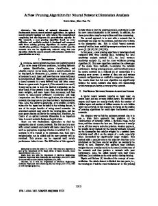
Fig. 1. Flow diagrams of (a) the cascaded and (b) the simultaneous inversion algorithms.

is a function of the unperturbed synthetic electric field in the space domain. We next substitute (9) into (4) and obtain ˆ t Es δε + Es δσ). δEs = G(∂

s

Esobs

where E (ε, σ) and are the synthetic and observed data, respectively, T indicates the transpose operator, and the sums are over sources s, receivers d, and observation times τ . We minimize the functional (7) using a gradient-type scheme based on an algorithm introduced in [41] which can be distilled into the following steps (see Fig. 1). 1) Select an initial model ε = εini and σ = σini (these can be defined by the results of prior ray tomographic inversions of the first-arrival times and maximum first-cycle amplitudes [42], [43]). 2) Compute the synthetic wavefields Es (ε, σ) using the initial model parameters. 3) Compute the update directions (the gradients in a steepest descent method) ∇Sε and ∇Sσ . 4) Compute the step lengths ζε and ζσ . 5) Update the model parameters using the steepest descent equations εupd = ε − ζε ∇Sε σupd = σ − ζσ ∇Sσ . 6) Set ε = εupd and σ = σupd , and repeat actions 2)–6) until convergence is achieved or until a specified number of iterations is reached.

(10)

(11)

The operator Ls that linearizes the forward problem with respect to small perturbations in the permittivity and conductivity values is defined as follows: δε s s s s s . E (ε + δε, σ + δσ) − E (ε, σ) = δE = [Lε Lσ ] δσ (12) Comparing (11) and (12) and expressing explicitly the kernel of Ls (see Appendix I-B) allow us to express the individual columns of Ls as follows: ˆ − x )∂t Es Lsε (x ) = Gδ(x

(13)

ˆ Lsσ (x ) = Gδ(x − x )Es .

(14)

The direct computation of the components of the sensitivity operator Ls would require as many solutions of the forward problem as there are model parameters. In any case, we will show in the next section that we are not directly interested in the sensitivity operator but only in its application to the residual, which requires just one solution of the forward problem. As the misfit function (7) does not consider the whole space–time domain of definition of the wavefields, in the remaining part of this paper, we will be interested in the operator Fs that

3394


linearizes the electric field at all the receivers and observation time combinations for each source δε [δEs ]d,τ = [Fsε Fsσ ] (15) δσ τ d

where [δEs ]d,τ = [Es (ε + δε, σ + δσ) − Es (ε, σ)]d,τ .

(16)

For the operator Fs , the columns are not as simply defined as for Ls . In the following, we will still be able to use, without any additional approximation, the simpler form of Ls instead of Fs for the computation of the gradient. of the range of Ls and Note that the range of Fs is a subset s s δε that the projection of [Lε Lσ ] δσ on the range of Fs equals δε . [Fsε Fsσ ] δσ

Since the columns of the sensitivity operator are the solution of a forward problem, we can leave the term containing the forward solution Es on the left side and apply the transpose of the Green’s operator to the residual. This avoids us from having to perform direct computation of the sensitivity operator, as foreshadowed in Section III-A. The aforementioned expressions are entirely general, allowing the inversion of various data sets (entailing any combination of source and receiver orientation, e.g., crosshole and borehole-to-surface). After some straightforward manipulations, we can express (22) as ˆ T Rs (δ(x − x )∂t Es )T G ∇Sε (x ) (23) = T ˆT s ∇Sσ (x ) (δ(x − x )Es ) G R s where the generalized residual wavefield Rs is given by Rs =

d

B. Gradients of the Misfit Function We have introduced the cost or objective function in the following form: 1 s S(ε, σ) = [E (ε, σ) − Esobs ]T d,τ 2 s τ d

· δ(x − xd , t − τ ) [Es (ε, σ) − Esobs ]d,τ .

(17)

As the gradient of the misfit function is defined by means of a first-order approximation, viz. δε + O(δε2 , δσ 2 ) S(ε + δε, σ + δσ) = S(ε, σ) + ∇S T δσ (18) using the same linearization as in (15), it is equivalent to FsT [ΔEs ]d,τ (19) ∇S = s

d

τ

where we have introduced the following notation for the residual wavefield: [ΔEs ]d,τ = δ(x − xd , t − τ )[Es (ε, σ) − Esobs ]d,τ .

(20)

Due to the properties of Ls and Fs as described at the end of Section III-A, it follows that FsT [ΔEs ]d,τ = LsT [ΔEs ]d,τ .

(21)

The gradients are then found by applying the transpose of Ls to the residual. More precisely, the single spatial components of the gradients are obtained by performing an inner product of the individual columns of Ls and the residual wavefield. For this reason, we have derived earlier the explicit expressions for the columns of Ls [(13) and (14)]. Using the results summarized in (13) and (14), these allow us to write the gradients as ˆ T [ΔEs ]d,τ ∇Sε (x ) (δ(x − x )∂t Es )T G . = T ˆT s ∇Sσ (x ) (δ(x − x )E ) G [ΔEs ]d,τ s τ d (22)

[ΔEs ]d,τ .

(24)

τ

In (23), Es indicates the solution of Maxwell’s equation in ˆ T Rs can be interpreted as a backwardthe medium, whereas G propagated vectorial field in the same medium (for details, see Appendix I-A). The simpler formula given by (23) shows that the gradient is found by summing the three-component inner products of the forward-propagated vectorial field and the backward-propagated residual vectorial field over all the sources. The inner product involves an integration over the ˆ T Rs . The presence of whole space–time domain of Es and G spatial delta functions δ(x − x ) corresponding to the spatial components of the gradients ∇Sε (x ) and ∇Sσ (x ) reduces the inner product to a zero-lag cross-correlation in time (see Appendix I-A). C. Step Lengths Once the gradients are found, step lengths are required to update the whole permittivity–conductivity model. Theoretically, the dielectric permittivities and electrical conductivities should be updated according to

ε ∇Sε εupd = −ζ · . σ σupd ∇Sσ

(25)

An optimal step length ζ can be found by following the approach introduced in [44], which involves searching for a minimum of the objective function along the direction of the gradient S(ε + ζ∇Sε , σ + ζ∇Sσ ).

(26)

The function in (26) has just one independent variable (i.e., the step length ζ), whereas ε, σ, ∇Sε , and ∇Sσ are fixed. The minimum is achieved simply by setting to zero the first derivative ∂S(ε + ζ∇Sε , σ + ζ∇Sσ ) = 0. ∂ζ

(27)

According to [44], the critical point occurs at the value given by (28) shown at the bottom of the next page.


3395

Here, Es (ε, σ) is the synthetic wavefield for the model parameter estimates (ε, σ), κ is an empirically established small number (see Appendix I-C for guidelines on how to choose such numbers), and Es (ε + κ∇Sε , σ + κ∇Sσ ) is the synthetic wavefield computed for perturbed permittivities and conductivities in the respective gradient direction [this process requires an additional finite-difference time-domain (FDTD) simulation]. Large differences between the permittivity and the conductivity sensitivities can cause this simultaneous inversion to fail for complex models. We quantified these differences by means of three numerical experiments which analyzed the differences between radargrams generated for a specific model (e.g., model 2 in Section V) and the same model perturbed in three different ways as follows: 1) combined permittivity/conductivity perturbations (E(ε + κ∇Sε , σ + κ∇Sσ ) − E(ε, σ)); 2) pure conductivity perturbation (E(ε, σ + κ∇Sσ ) − E(ε, σ)); 3) pure permittivity perturbation (E(ε + κ∇Sε , σ) − E(ε, σ)). These tests showed that there is a two order of magnitude difference between the conductivity-only variation and the other two, which look very similar. The step length is therefore determined by the permittivity gradient in such a scheme. Ernst et al. [37] proposed a stepped or cascaded inversion that involves inverting for the permittivities while keeping the conductivities fixed (constant) for a certain number of iterations and then analogously inverting for the conductivities while keeping the permittivities fixed. In order to minimize the effects of conductivity anomalies during the permittivity inversions, a normalized version of the data residual was exploited by dividing through by the energy in the modeled traces, while the ordinary residual was used for the conductivity inversions. The reader is referred to [37] for details. By contrast, Tarantola [45] suggests updating different types of model parameters according to different step lengths. In the GPR case, this becomes [εupd ] = [ε] − ζε · [∇Sε ]

(29)

[σupd ] = [σ] − ζσ · [∇Sσ ].

(30)

We present here a quasi-simultaneous inversion that updates the permittivities and the conductivities at each iteration by

s

ζ = κ s

d

τ

d

τ

searching for critical points separately along the ∇Sε and ∇Sσ directions S(ε + ζε ∇Sε , σ)

(31)

S(ε, σ + ζσ ∇Sσ ).

(32)

The two critical points of (31) and (32) occur at the values given by (33) and (34), shown at the bottom of the page, where κε and κσ are two different small stabilizing numbers. Note that the small stabilizers κε and κσ in (33) and (34) must be chosen carefully between upper and lower limits (see Appendix I-C for details). These stabilizing numbers may need to be updated during the inversion process as a consequence of the variations in the gradient amplitudes [44]. In our numerical experiments, values of κε = 10−5 and κσ between 1 and 25 were found to be appropriate. Although this newly introduced process requires an additional forward model calculation, the simultaneous nature of the process results in a reduction in the total number of required FDTD calculations because it updates both the permittivity and conductivity distributions at each iteration [see Fig. 1]. Our full-waveform inversion scheme requires the forward problem to be solved four times per iteration at each transmitter location: once to evaluate the synthetic data, once to compute the update in both gradient directions, and twice to determine the step lengths. By comparison in [37], different residuals were used such that the permittivity and conductivity gradients could not be computed with a single forward model calculation and six forward solutions were needed. In addition, while the cascaded scheme requires the user to select or choose the number of permittivity/conductivity iterations to be executed before updating the permittivity/conductivity, the simultaneous inversion does not. As a result, the implementation of the simultaneous inversion scheme is simpler. The differences between the algorithm employed by Ernst et al. [37] and the new inversion scheme are highlighted in the processing flow chart of Fig. 1. This diagram is for ten iterations, but it can be extended to any number. It involves ten simultaneous updates of permittivity and conductivity requiring 40 forward model computations. This can be compared to ten permittivity updates followed by ten conductivity updates with the cascaded scheme involving 60 forward model runs. The solutions are not the same in each case. Note that the simultaneous scheme only involves 2/3 of the computational effort.

s s [Es (ε + κ∇Sε , σ + κ∇Sσ ) − Es (ε, σ)]T d,τ δ(x − xd , t − τ ) [E (ε, σ) − Eobs ]d,τ

s s [Es (ε + κ∇Sε , σ + κ∇Sσ ) − Es (ε, σ)]T d,τ δ(x − xd , t − τ ) [(E (εκ∇Sε , σ + κ∇Sσ )) − E (ε, σ)]d,τ (28)

s

ζε = κε

d

τ

s s [E(ε + κε ∇Sε , σ) − Es (ε, σ)]T d,τ δ(x − xd , t − τ ) [E (ε, σ) − Eobs )]d,τ

s s [Es ((ε + κε ∇Sε , σ) − Es (ε, σ)]T d,τ δ(x − xd , t − τ ) [E ((ε + κε ∇Sε , σ) − E (ε, σ)]d,τ T s s s s s d τ [E (ε, σ + κσ ∇Sσ ) − E (ε, σ)]d,τ δ(x − xd , t − τ ) [E (ε, σ) − Eobs )]d,τ ζσ = κσ T s s s s s d τ [E ((ε, σ + κσ ∇Sσ ) − E (ε, σ)]d,τ δ(x − xd , t − τ ) [E (ε, σ + κσ ∇Sσ ) − E (ε, σ)]d,τ s

d

(33)

τ

(34)

3396


D. Different Parameterizations of the Physical System We have presented here the derivation of the inversion algorithm based on the natural parameters ε, σ, and μ0 . Different parameterizations (i.e., changes of coordinates in the model space) can, however, be easily implemented. A logarithmic representation for the permittivity and the conductivity is normally used as follows:

ε(x) (35) εˆ(x) = log ε0

σ(x) σ ˆ (x) = log (36) σ0 where ε0 is the vacuum permittivity and σ0 is an arbitrary conductivity value, in our case 1 S/m. The choice of logarithmically scaled parameters is particularly important for the inversion because it conveys to the model space the structure of a linear space [45]. In addition, this parameterization ensures positive values of permittivity and conductivity and allows compression of model values to accommodate a much wider range [35]. A change of model representation for the inversion process affects just the formula of the gradient directions. First, we introduce a new representation for the objective function ε, σ ˆ) S (ε(ˆ ε), σ(ˆ σ )) = S (ˆ

(37)

and then, we express the new gradients ∇Sεˆ and ∇Sσˆ as functions of ∇Sε and ∇Sσ , whose values are expressed in (23) ∂S ∂ε ∂S = ∂ εˆ ∂ε ∂ εˆ

∂S ∂σ ∂S = . ∂σ ˆ ∂σ ∂ σ ˆ

(38)

By using the definition given by (35) and (36), we find

∇Sεˆ (x ) ∇Sσˆ (x )

ε(x )∇Sε (x ) = . σ(x )∇Sσ (x )

the frequency content of the sources. The usual requirement is to have at least ten grid points per minimum wavelength in the model [47]. In our models, we employed a pulse with a dominant frequency of about 160 MHz, so we had to use a grid spacing of 2 cm, leading to 105 − 106 grid points per model. Given the source–receiver distances involved in the models, we required a few thousand time steps to achieve the 150-ns-long waveforms and, at the same time, to satisfy the stability criteria with respect to the time sample interval. Generalized perfectly matched layers, 40 cells in width, were applied at the edges of the domain to suppress artificial grid boundary reflections [49]. For the computation of the update directions, the complete Ex and Ez fields generated by all transmitters at all grid locations need to be kept in memory. This would require a huge core memory of about 40 × Nsrc GB, where Nsrc is the number of transmitters. However, since the spatial resolution that we can expect on the model is much lower than the discretization needed for accurate forward modeling, multiple forward cells can be represented with a single inversion cell. In all our models, we include 3 × 3 forward cells within one inversion cell without significant loss of resolution in the inversion process [37]. This reduces the memory requirements by roughly an order of magnitude and avoids memory-swapping procedures in realistic situations. Since the single transmitter calculations are independent of each other, the computation scheme can be implemented efficiently on a distributed computer cluster, comprising ideally one slave CPU per transmitter and a single master CPU. The extra costs due to data distribution are only about 10% relative to the computation of a forward solution. Accordingly, the total computational time Tcomp required for a complete simultaneous inversion, if memory-swapping is avoided, is given by Tcomp ≈ 4 · 1.1 · Tforward · Niter

(39)

IV. I MPLEMENTATION The theory presented so far is entirely general and can be applied to 3-D or 2-D problems. However, the computing resources needed to simulate many multiple forward calculations in 3-D using an FDTD scheme [46] are prohibitively expensive at the present time. We therefore test our inversion scheme in laterally invariant (2-D) media with line sources (in y-direction) in a Cartesian coordinate frame. Assuming no medium property variations in the y-direction, the six components of the EM field are decoupled into two independent sets of equations [47]. We can then solve for just one of these sets. For a borehole configuration, we solve Maxwell’s equations for the TEy mode, (i.e., the mode whose electric field is always transverse to the y-direction [48]) which involves the following field components: Ex , Ez , and Hy . Note that, theoretically, the algorithm can deal with all source and receiver combinations at the same time. However, this is currently not feasible in a practical sense. To ensure stability and avoid numerical grid dispersion in our simulations, we had to consider the medium properties and

where Tforward is the time required for a single forward calculation and Niter is the number of iterations. V. S YNTHETIC R ESULTS A. Application to Synthetic Data In the following, we refer to “borehole” and “surface” receivers and transmitters. A “borehole” receiver is defined here as an antenna that senses the vertical component of the electric field Ez , whereas a “surface” receiver detects the horizontal component Ex . Similarly, we have defined ’borehole’ transmitters. For comparison purposes, very similar models to those used in [37] are employed here. For convenience, we use the relative permittivity εr = ε/ε0 or dielectric constant, rather than the absolute permittivity. The synthetic antennas in our simulations have a central frequency of 160 MHz and a bandwidth of about three octaves, which corresponds to wavelengths of 25–280 cm within the background medium (the wavelengths get significantly smaller in the high permittivity inclusions) and a dominant wavelength of about 1 m. In order to focus the sensitivity on the interwell medium rather than in proximity of the sources and receivers, the gradient had to be downscaled close to the antennas. In addition, values of the gradient at cells in the areas between the model borders and the


3397

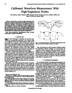
Fig. 2. (a) Relative permittivity of model 1. Relative permittivity tomograms that result from applying (b) crosshole ray-based, (c) crosshole simultaneous fullwaveform, and (d) three-sided simultaneous full-waveform inversion schemes to noise-free traces generated by model 1. (e) A −A permittivity sections through tomograms in (a)–(d). (f) B −B permittivity sections through tomograms in (a)–(d).

antennas, as well as at the top and bottom areas, are set to the average of the neighboring gradient values. Furthermore, a low-pass (smoothing) Gaussian filter was applied to the

gradient over the whole domain. At any point P = (x, y) of the domain, the gradient used to update the model was assigned a value given by a weighted mean of the gradient at P and at

3398


Fig. 3. Selection of radargrams generated by the source placed at 4-m depth in model 1. The red traces correspond to the synthetic observed traces, the blue traces are the synthetic response of the model obtained by applying conventional travel-time tomography to noise-free data, and the traces generated by the final model obtained by applying borehole full-waveform inversion are displayed in dashed black and practically overlie the red traces. The match, in data space, between the red and dashed black traces is much better than that between the red and blue ones. The different fits between the data should be compared to the differences in the model space between the respective tomograms [see Fig. 2(b) and (c)].

the adjacent eight points. The weight of the central point P was twice that of the points along the horizontal–vertical directions and four times that of the points along the diagonals. B. Example 1: Single Small Cylindrical Body of Anomalous Permittivity The first model includes an isolated cylindrical body of circular 2-D cross section (e.g., a pipe) sitting in a homogeneous host rock of relative permittivity εr = 4 and conductivity σ = 0.1 S/m [see Fig. 2(a)]. The body is anomalous in permittivity only (εr = 5), having the same conductivity as the host rock. It is a rather small object of 0.5 m in diameter located in the center of the target field between two 10-m-deep boreholes which are 10 m apart. Twenty-one transmitter positions, indicated by the crosses in Fig. 2, are spaced at 0.5-m intervals in the left borehole, and 21 receiver positions, indicated by the open circles, are spaced at 0.5 m in the right borehole. Synthetic radargrams were numerically generated for this crosshole experiment [37], [38], [50] and constituted the input data for the first set of inversions. Fig. 3 shows a representative shot gathered for a transmitter at 4-m depth. The observed data are shown in red. The image produced by first-arrival-time ray tomography is shown in Fig. 2(b). It is a blurred picture with practically no evidence of the anomalous feature. Far superior results were obtained using full-waveform inversion. The cascaded scheme used the correct conductivity values during the whole permittivity inversion, whereas the simultaneous scheme used the correct conductivity as a starting value and also inverted for the conductivity. The cascaded scalar inversion (not shown here) and the simultaneous vectorial crosshole inversion [Fig. 2(c)] yield similarly improved permittivity images of the target but with some spreading in the horizontal direction. There is also

some butterfly-pattern blurring associated with the limited angular coverage afforded by such a recording geometry and a homogeneous background (no additional backscattering is possible to increase the target coverage). Despite the updating of the conductivity at every iteration step, the simultaneous inversion proved to be very stable and, in fact, returned an almost homogeneous conductivity medium of the correct value (results not shown here). The small-scale conductivity fluctuations for the inverted noise-free data were on the order of a few thousands of millisiemens per meter or less than 2%. For the three-sided inversion experiment, an additional 12 receivers were simulated along the ground surface and transmitters placed in both boreholes at 0.5-m spacing [see Fig. 2(d)]. As foreshadowed in Section III-B, the vectorial algorithm could be employed to invert the more extensive crosshole/boreholeto-surface synthetic data set [Fig. 2(d)]. The reconstruction of the anomalous body is significantly improved in both shape and amplitude. Fig. 2(e) and (f) shows the recovered relative permittivity cross sections along the horizontal and vertical lines A −A and B −B through the center of the target for all three inversions as well as the true model. The crosshole inversion yields a maximum relative permittivity of 4.5 for the body, compared to the three-sided inversion which gives a value of approximately five, very close to the true value. Fig. 3 shows the computed radargrams (dashed black lines) for the final inverted model, superimposed on the original traces (red traces). The waveforms match remarkably well. The blue traces show the computed traces for the initial ray-based model, which show a mismatch in both amplitude and phase relative to the actual data (red traces). Next, we added Gaussian random noise of up to 5% to the synthetic traces prior to inversion. Results for noisecontaminated crosshole and three-sided recording experiments are shown in Fig. 4. The images are slightly different compared to the noise-free case [Fig. 2(c) and (d)], but the small circular target is again well recovered. The most prominent difference between Figs. 2 and 4 is the background ripple effect in the latter. The small-scale fluctuations of maximum wavelength equal to the trace spacing are equally distributed as alternating high and low features of magnitude less than 7% in Fig. 4. The ripple is less pronounced in the three-sided imaging result. The permittivity profiles through the central anomalous body in Fig. 4(c) and (d) again show the fidelity of the recovered image in both size and shape. C. Example 2: Two Small Cylindrical Bodies of Dissimilar Anomalous Conductivity and Permittivity The permittivity and conductivity images obtained by inverting the first-arrival times and the first-pulse peak amplitudes are quasi-homogeneous, with no evidence for the embedded inclusions [see Fig. 5(b) and (h)]. The situation improves markedly when waveform inversion is performed. Both stepped (cascaded) scalar and simultaneous vectorial inversions were conducted. but we only show the results for the latter [Fig. 5(c) and (i)]. The resistive feature is not imaged, as well as the conductor in the conductivity tomogram, due to its limited data sensitivity. Fig. 6 shows that the simultaneous scheme reached convergence in the data space


3399

Fig. 4. Relative permittivity tomograms that result from applying (a) crosshole simultaneous full-waveform and (b) three-sided simultaneous full-waveform inversion schemes to traces generated by model 1 [Fig. 2(a)] contaminated by 5% Gaussian noise. (c) A −A permittivity sections through tomograms in (a)-(b). (d) B −B permittivity sections through tomograms in (a)-(b).

after 30 iterations (corresponding to calculating 120 model runs), while the stepped scheme needed 44 permittivity and 33 conductivity updates in order to achieve a comparable data misfit (corresponding to calculating 231 model runs). The cascaded inversion shows that, for every separate permittivity or conductivity inversion, a certain plateau is reached due to the fact that the conductivity or permittivity is fixed. By contrast, for the simultaneous inversion, the root-meansquare (rms) curve shows a very smooth and faster convergence. For the three-sided experiment, in which additional 12 receivers were simulated along the surface and an additional 21 transmitters in the right borehole, the vectorial inversion produced significantly improved permittivity and conductivity images [see Fig. 5(d) and (j)]. In order to improve convergence and focus the sensitivity on the area of interest, just part of the data was inverted. Only those traces for source–receiver distances comparable to the borehole separation could be utilized; otherwise, the

dynamic range would have been totally captured by the very strong near-source arrivals. Both the high- and low-permittivity bodies are better reconstructed in shape and magnitude compared to the crosshole data set inversion alone. In addition, the resolution of the conductivity anomalies is noticeably increased when the complete data set (crosshole and boreholeto-surface) is inverted. This is best seen in Fig. 5(e) and (f), which shows the reconstructed permittivity and conductivity values along the diagonal lines A −A and B −B through the model and tomograms. Although the shape is well recovered, the conductivity for the resistive body falls well short of its true value. To appreciate the goodness of data fit for the final inverted model, we show the computed traces (dashed black lines) superimposed on the observed data (red lines) for transmitter position at 4 m, left borehole, in Fig. 7. Again, the match is good and significantly better than the traces computed for the ray-based starting model, shown in blue.

3400


Fig. 5. (a) Relative permittivity and (g) conductivity distributions of model 2. Relative permittivity and conductivity tomograms that result from applying [(b) and (h)] crosshole ray-based, [(c) and (i)] crosshole simultaneous full-waveform, and [(d) and (j)] three-sided simultaneous full-waveform inversion schemes to noise-free traces generated by model 2. (e) A −A permittivity sections through tomograms in (a)–(d). (f) B −B conductivity sections through tomograms in (g)–(j). The open black circles in the central part of each diagram indicate the true position and size of the anomalous bodies.

but in similar fashion to the first example, there exist small-scale fluctuations in the tomograms associated with the noise and star blurring of the anomalous bodies caused by incomplete angular and spatial sampling. D. Example 3: Layered and Stochastic Media With Multiple Embedded Cylindrical Inclusions

Fig. 6. Normalized rms curves for the cascaded (in blue and green are the permittivity and conductivity inversion intervals, respectively) and the simultaneous (in red) inversion schemes.

The inversions were repeated for synthetic traces contaminated by 5% Gaussian noise. The anomalous features are still clearly distinguishable from the background [see Fig. 8(a)–(f)],

Our third and final example involves a far more complicated model, comprising a three-layered structure of contrasting permittivities and conductivities with superimposed stochastic variations and multiple embedded inclusions (see Fig. 9). The 3-m-thick top layer has an average relative permittivity εr = 5.2 and an average conductivity σ = 2.8 mS/m. The middle layer has an undulating lower boundary from 15.5- to 17-m depth. It is characterized by an average relative permittivity εr = 3.7 and average conductivity σ = 2.0 mS/m. The basal unit has an average relative permittivity εr = 5 and an average conductivity σ = 0.1 mS/m. The standard deviations on εr and σ in these stochastic media are 0.1 and 0.5 mS/m, respectively, with correlation lengths in the horizontal and vertical directions of 1.0 and 0.2 m. Three small (0.5-m-diameter) cylindrical bodies separated horizontally by 2 m occur at 6.5-m depth within layer 2. A fourth much larger cylindrical inclusion


Fig. 7. Selection of radargrams generated by the source placed at a 4-m depth in model 2. The red traces correspond to the synthetic observed traces, the blue traces are the synthetic response of the model obtained by applying conventional travel-time tomography to noise-free data, and the traces generated by the final model obtained by applying borehole full-waveform inversion are displayed in dashed black (they practically overlie the red traces). The match, in data space, between the red and dashed black traces is much better than that between the red and blue ones. The different fits between the data should be compared to the differences in the model space between the respective tomograms [see Fig. 5(b)–(h) and (c)–(i)].

of 2 m in diameter occurs at position (4, 12). All bodies are moderately conductive with σ = 10 mS/m and of high relative permittivity εr = 80 equal to that of water. The cylindrical anomalies could be, for example, fluid-filled pipes and a fluidfilled tunnel. The structure is straddled by two vertical 20-mdeep boreholes set 10 m apart. Forty-one equally spaced transmitter positions (0.5-m increment, indicated by white crosses in Fig. 9) are located in the left borehole, and 41 receivers (indicated by white circles) are located in the right borehole (see Fig. 9). Full-waveform synthetic radargrams generated for this structure constitute the input data for the various inversions. A representative shot gathered for a transmitter at a 10-m depth is shown in Fig. 10. Results of the ray-based tomography applied to first-arrival times and amplitudes are shown in Fig. 9(b) and (g) for the permittivity and conductivity, respectively. The three layers are essentially recovered in the permittivity image, but it is hard to discern the boundaries in the conductivity image. The largest inclusion is recognizable on the permittivity tomogram, but its shape and magnitude are poorly recovered. The conductivity tomogram shows just a slight increase over the background value for the three embedded smaller bodies, but they cannot be separately resolved. The image is just an indistinct blur. The largest inclusion is also manifest as a localized but severely distorted representation of a slightly more conductive feature. In addition, three artificial resistive bodies have been introduced as image artifacts. Fig. 9(c) and (h) shows the results for the cascaded vectorial full-waveform inversion of the crosshole data, whereas results for the simultaneous vectorial inversion are shown in Fig. 9(d) and (i). The cascaded inversion first fixes (holds constant) the conductivity and inverts for permittivity. It then fixes this inverted permittivity result and inverts for the conductivity

3401

distribution. The process can be repeated over several cycles. By contrast, the simultaneous inversion solves for permittivity and conductivity at the same time, without holding either one fixed. Both schemes yield tomograms far superior to the ray-based result, particularly the conductivity tomograms, which now reveal all four inclusions as distinct resolvable features. The simultaneous vector inversion does a better job in recovering the boundaries between the three layers on the permittivity tomogram; in particular, the cascaded vectorial inversion yields an erroneous upward curving boundary for the top interface [Fig. 9(c)]. The cascaded vectorial inversion also overestimates the conductivity contrasts of the four conductive inclusions [compare Fig. 9(h) with the true model, Fig. 9(f)], whereas the simultaneous vector tomogram [Fig. 9(i)] only slightly overshoots the real values. Surprisingly, the cascaded vectorial inversion does a better job in separating the three embedded conductors at a depth of 6 m. Neither of these waveform inversions outperforms ray tomography in recovering the tunnel feature on the permittivity image. Both waveform inversions required comparable CPU time but have somewhat different stability criteria. For the cascaded inversion, three different starting models were used: two for the first permittivity inversion cycle based on the ray tomography results (from first-arrival times and initial maximum pulse amplitudes) and a different homogeneous conductivity distribution for the first conductivity inversion cycle. The application of the simultaneous inversion required just two starting models: the travel-time tomography result for the permittivity distribution and a homogeneous conductivity distribution. Furthermore, the cascaded scheme was not as stable as the simultaneous scheme. Small high-conductivity artifacts between the second and the third layers in the conductivity image were generated during the inversion process. We could have avoided these problems by applying smoothing to the model or setting constraints on the conductivity image, but this would have worsened the clear separation between the pipes. On the other hand, the simultaneous scheme was not troubled by spurious features. In keeping with the other examples, we also simulated an additional set of 12 receivers along the top surface of the model and an additional set of transmitters in the right borehole [see Fig. 9(e) and (j)] and synthesized the data for this combined crosshole/borehole-to-surface experiment. As for previous models, the very short offset waveform data were excluded from inversion using the simultaneous vector algorithm. Results are shown in Fig. 9(e) and (j). They are, by far, the best tomograms that result from the various approaches. The individual small conductors are now clearly separated. The shapes of all embedded bodies are essentially recovered. A detailed comparison can be made in Fig. 9(k), which shows the profiles from all four inversions along the horizontal line A−A which passes through the embedded anomalies. The true conductivity profile is also given for reference. Although the maximum conductivity of the anomalous bodies is overestimated by the three-sided inversion, the peak-to-trough size of the anomaly between the bodies matches quite closely the actual variation from the background. This overestimation may be caused by underestimating the relative permittivity anomaly [see Fig. 9(e)]. In providing a proper damping factor, the simultaneous algorithm has a tendency to compensate and therefore overshoot the

3402


Fig. 8. Relative permittivity and conductivity tomograms that result from applying [(a) and (b)] crosshole simultaneous full-waveform and [(c) and (d)] threesided simultaneous full-waveform inversion schemes to traces generated by model 2 [Fig. 5(a) and (g)] contaminated by 5% Gaussian noise. (e) A −A permittivity sections through tomograms in (a)–(d). (f) B −B conductivity sections through tomograms in (g)–(j). The open black circles in the central part of each diagram indicate the true position and size of the anomalous bodies.

correct conductivity value. Fig. 10 compares the computed traces for the final inverted model (dashed black traces) and the starting model (blue traces) with the actual observed data

(red traces). Note the significant improvement in matching the waveforms as the inversion proceeds. The presence of conductive anomalies has an appreciable effect on the amplitudes


3403

Fig. 9. (a) Relative permittivity and (f) conductivity distributions of model 3. Relative permittivity and conductivity tomograms that result from applying [(b) and (g)] crosshole ray-based, [(c) and (h)] crosshole stepped (cascaded) full-waveform, [(d) and (i)] crosshole simultaneous full-waveform, and [(e) and (j)] three-sided simultaneous full-waveform inversion schemes to noise-free traces generated by model 3. (k) A −A sections through the conductivity tomograms in (f)–(j).

in particular, which are not incorporated nearly as well in the computed traces for the starting model (no conductivity anomalies). VI. C ONCLUSIONS We have presented a new vector algorithm for the inversion of full-waveform GPR data that updates permittivity and conductivity simultaneously. The new inversion scheme is highly versatile and can be applied to data collected with

any source–receiver setup. The algorithm has been derived by solving Maxwell’s equations and using a vectorial fullwavefield notation that simplifies the derivation of the gradient direction as a zero-lag cross-correlation of forward- and backward-propagated vector fields. An FDTD code based on the new algorithm and optimized for implementation on PC clusters was applied to a number of synthetic 2-D models with realistic permittivity–conductivity distributions and source wavelets to invert crosshole and surface-to-borehole data. The tests presented here, along with many more not shown, allow

3404


whose explicit representation in index form is s (xd , τ ))i . Tks,d,τ (x , t ) = Gik (xd , τ, x , t ) (E s (xd , τ ) − Eobs (A3)

The formalism of (A3) is different from that in (A1). Apart from the missing integration over space and time [we consider the source to be a delta function in space and time, so an integration takes place in (A3)], the indices of the Green’s function are differently related to the index of the source, and the space–time variables are switched. To be able to better interpret (A3), we begin by taking advantage of reciprocity; we know that reciprocity can be expressed in terms of Green’s functions as [51] Gik (xd , τ, x , t ) = Gki (x , τ, xd , t ). Fig. 10. Selection of radargrams generated by the source placed at a 10-m depth in model 3. The blue traces are the synthetic response of the model obtained by applying conventional travel-time tomography to noise-free data, whereas the traces generated by the final model obtained by applying borehole full-waveform inversion are displayed in dashed black. Finally, the red traces correspond to the synthetic observed traces. The match, in data space, between the dashed black and the red traces is not as good as for model 1 (Fig. 3) and model 2 (Fig. 7). Nevertheless, it is still far better than the match between the blue and the red traces. The different fits between the data should be compared to the differences in the model space between the respective tomograms [see Fig. 9(b)–(g) and (d)–(i)].

us to assert that the results using the new algorithm are a significant improvement over previous approaches based on a scalar formulation and a cascaded updating of the permittivity and conductivity distributions. A PPENDIX I D ETAILS ON THE I NVERSION A LGORITHM

The transpose of an integral operator is defined by means of its kernel. A linear operator and its transpose have the same kernels, the only difference being in the variables of the summation/integration, which are complementary [45]. ˆ on We have defined earlier the action of the operator G ˆ T , we a source function J. To give a clear explanation of G ˆ For a source J, receiver d, and need to explore in detail G. observation time τ , (5) is explicitly written for each component (i = x, y, z) of the electric field as =

T

dV (x ) V

dt Gik (x, t, x , t )Jks (x , t ). (A1)

0

It is important here to note the positions of all the variables and the indices of the Green’s functions, the source, ˆ acts by summing over the and the solution. The operator G whole spatial and temporal domains to yield a function at a ˆ T acts from that given specific time–position. The transpose G time–position to give a function defined in the whole spatial and temporal domain. We define now a new vector function T as the result of the application of GT to the residual [ΔEs ]d,τ as required in (22) ˆ T [ΔEs ]d,τ Ts,d,τ = G

Thus, we rewrite (A3) as s (xd , τ ))i . Tks,d,τ (x , t ) = Gik (xd , τ, x , t ) (E s (xd , τ ) − Eobs (A5)

This helps us to interpret the residual as a source for a propagation problem. In fact, both the spatial components and the indices of the tensor Gki are related to those of the vector s (xd , τ ))i in (A5) as they are related to the (E s (xd , τ ) − Eobs source term in (A1). Our problem is time invariant. This means that the Green’s tensor satisfies the following relation: Gki (xd , τ, x , t ) = Gki (xd , τ − t , x , 0).

(A6)

This allows us to rewrite (A5) as

ˆ A. Transpose of G

Eis (x, t)

(A4)

(A2)

s Tks,d,τ (x , t ) = Gki (x , τ −t , xd , 0) (E s (xd , τ )−Eobs (xd , τ ))i (A7)

and to interpret Tks,d,τ (x , t ) as being the solution of a propagation problem where the source is the residual s (xd , τ ))i that is back propagated in time (as (E s (xd , τ ) − Eobs t is decreasing, the argument τ − t increases). We introduce Ts,d,τ in compact notation for the threecomponent wavefield in (A7). We can now look upon (22) as (δ(x − x )∂t Es )T Ts,d,τ ∇Sε (x ) (A8) = ∇Sσ (x ) (δ(x − x )Es )T Ts,d,τ s τ

d

or expanding out, we obtain ∇Sε (x ) ∇Sσ (x)

T dV(x) dt δ(x−x ) ∂t Es(x, t )·Ts,d,τ(x, t ) 0 V = . s

T s,d,τ s d τ dV(x) dt δ(x−x ) E (x, t )·T (x, t ) V

0

(A9) This is equivalent to a zero-lag cross-correlation in the time domain of the forward- and backward-propagated vectorial


3405

fields at any point in the model space

These are equivalent to

T dt ∂t Es (x , t )·Ts,d,τ (x , t ) ∇Sε (x ) 0 = .

T s ∇Sσ (x ) s,d,τ s τ d dt E (x , t )·T (x , t )

[Lsε (x )]x,t

0

[Lsσ (x )]x,t

By using the distributive property, we can move the sums over d and τ in the integral in (A10) and finally obtain ⎛T ⎞ s,d,τ s ∂ dt E (x , t )· T (x , t ) t d τ ⎟ ∇Sε (x ) ⎜ ⎜0 ⎟. = T ⎝ s s,d,τ ⎠ ∇Sσ (x ) s dt E (x , t )· d τ T (x , t )

δE (x, t) =

T

dV (x ) +

dV (x )

dt G(x, t, x , t )Es (x , t )δσ(x )

where t is any point in time, x is any domain point, and the field Es is generated by a particular (given) source. δEs (x, t) = dV (x ) [Lsε (x )]x,t δε(x ) +

dV (x ) [Lsσ (x )]x,t δσ(x ).

(A13)

V

The equivalence of (A12) and (A13) holds for Ls defined in terms of its components as follows: [Lsε (x )]x,t

T =

dt G(x, t, x , t )∂t Es (x , t )

(A14) ACKNOWLEDGMENTS

0

[Lsσ (x )]x,t =

T

(A17)

Similar arguments apply when we consider the multiple step lengths ζε and ζσ and multiple stabilizers κε and κσ [see (33) and (34)]. We carried out an investigation of the sorts of results that can arise depending on the choice of κ, using the values 10−15 , 10−10 , 10−5 , and 10, and data from model 2. The intermediate choices of κ, i.e., 10−10 and 10−5 , yielded similar waveforms. This trend is achieved when the choices of κ satisfy both the linearity range condition and round-off truncation errors, as indicated in (A18). Results are considerably different from the other two cases when κ is 10−15 and 10. When 10−15 is chosen, the computation suffers from truncation (round-off) errors associated with very small quantities, while when κ is 10, the linearity condition is violated. Similar considerations are also valid for the numbers κε and κσ .

(A12)

V

0

1) κ has to be small enough so that the perturbed model still s lies in the linearity range of Es (ε, σ)E + κ∇Sε , σ + ∇Sε(ε s s T κ∇Sσ ) − E (ε, σ) ≈ ∇E (ε, σ) κ ∇Sσ . 2) κ has to be large enough to avoid truncation (round-off) errors when dealing with small numbers in the computer.

0

V

(A16)

The constant κ in (28) has to be chosen so that the linear approximation of the forward problem holds [44]. Expanding out to first order, we rewrite (28) as (A18), shown at the bottom of the page. If E was a linear function of (ε, σ), the remainder would be zero, and ζ would be independent of κ because all the κ terms would cancel out. Since κ has to be chosen so that the linear approximation holds, it has to satisfy two different conditions as follows.

dt G(x, t, x , t )∂t Es (x , t )δε(x ) T

0

· (δ(x − x )∂t Es (x , t )) T = dV (x ) dt G(x, t, x , t )

C. Choice of the Small Number(s) κ in the Step Length(s)

0

V

dt G(x, t, x , t )

through the property of integrating a delta function. They are written in compact form as (13) and (14).

(A11)

T

· (δ(x − x )Es (x , t ))

Here, we derive the results presented in Section III-A conˆ In order to identify cerning the components of the kernel of L. ˆ the kernel of L, we need to interpret (11) as (12), i.e., as an integration over the model space. We rewrite (11) using the formalism presented in (5) as

dV (x )

V

ˆ B. Kernel of L

s

= V

(A10)

0

dt G(x, t, x , t )Es (x , t ).

The authors would like to thank the ETH Computer Services for allowing them access to the Brutus high-performance cluster.

(A15)

0

∇Sε T

δ(x − xd , t − τ ) [Es (ε, σ) − Esobs ]d,τ ζ ≈ κ

T

s (ε, σ)T δ(x − x , t − τ )κ ∇Sε sT (ε, σ)κ ∇Sε δ(x − x , t − τ ) ∇E ∇E d d s d τ ∇Sσ ∇Sσ s

d

τ

∇Es (ε, σ)T κ

∇Sσ

d,τ

d,τ

d,τ

(A18)

3406


R EFERENCES [1] G. Grandjean, J. C. Gourry, and A. Bitri, “Evaluation of GPR techniques for civil-engineering applications: Study on a test site,” J. Appl. Geophys., vol. 45, no. 3, pp. 141–156, Oct. 2000. [2] C. P. Kao, J. Li, Y. Wang, H. C. Xing, and C. R. Liu, “Measurement of layer thickness and permittivity using a new multilayer model from GPR data,” IEEE Trans. Geosci. Remote Sens., vol. 45, no. 8, pp. 2463–2470, Aug. 2007. [3] F. Soldovieri, J. Hugenschmidt, R. Persico, and G. Leone, “A linear inverse scattering algorithm for realistic GPR applications,” Near Surf. Geophys., vol. 5, no. 1, pp. 29–41, Feb. 2007. [4] K. C. Ho, L. Carin, P. D. Gader, and J. N. Wilson, “An investigation of using the spectral characteristics from ground penetrating radar for landmine/clutter discrimination,” IEEE Trans. Geosci. Remote Sens., vol. 46, no. 4, pp. 1177–1191, Apr. 2008. [5] R. Knight, “Ground penetrating radar for environmental applications,” Annu. Rev. Earth Planet. Sci., vol. 29, pp. 229–255, 2001. [6] A. Binley, P. Winship, R. Middleton, M. Pokar, and J. West, “Highresolution characterization of vadose zone dynamics using cross-borehole radar,” Water Resour. Res., vol. 37, no. 11, pp. 2639–2652, Nov. 2001. [7] A. Binley, G. Cassiani, R. Middleton, and P. Winship, “Vadose zone flow model parameterisation using cross-borehole radar and resistivity imaging,” J. Hydrol., vol. 267, no. 3/4, pp. 147–159, Oct. 2002. [8] J. Tronicke, K. Holliger, W. Barrash, and M. D. Knoll, “Multivariate analysis of cross-hole georadar velocity and attenuation tomograms for aquifer zonation,” Water Resour. Res., vol. 40, no. 1, p. W01 519, Jan. 2004. [9] M. C. Looms, K. H. Jensen, A. Binley, and L. Nielsen, “Monitoring unsaturated flow and transport using cross-borehole geophysical methods,” Vadose Zone J., vol. 7, no. 1, pp. 227–237, Feb. 2008. [10] N. Linde, A. Binley, A. Tryggvason, L. B. Pedersen, and A. Revil, “Improved hydrogeophysical characterization using joint inversion of crosshole electrical resistance and ground-penetrating radar traveltime data,” Water Resour. Res, vol. 42, no. 12, p. W12 404, Dec. 2006. [11] S. Hubbard, J. S. Chen, K. Williams, J. Peterson, and Y. Rubin, “Environmental and agricultural applications of GPR,” in Proc. 3rd Int. Workshop Adv. Ground Penetrating Radar, 2005, pp. 45–49. [12] L. Weihermuller, J. A. Huisman, S. Lambot, M. Herbst, and H. Vereecken, “Mapping the spatial variation of soil water content at the field scale with different ground penetrating radar techniques,” J. Hydrol., vol. 340, no. 3/4, pp. 205–216, Jul. 2007. [13] S. Lambot, E. C. Slob, I. van den Bosch, B. Stockbroeckx, and M. Vanclooster, “Modeling of ground-penetrating radar for accurate characterization of subsurface electric properties,” IEEE Trans. Geosci. Remote Sens., vol. 42, no. 11, pp. 2555–2568, Nov. 2004. [14] J. Huisman, J. Redman, and A. Annan, “Measuring soil water content with ground penetrating radar: A review,” Vadose Zone J., vol. 2, no. 4, pp. 476–491, Nov. 2003. [15] J. M. Carcione, “Ground radar simulation for archaeological applications,” Geophys. Prospect., vol. 44, no. 5, pp. 871–888, Sep. 1996. [16] J. A. Baker, N. L. Anderson, and P. J. Pilles, “Ground-penetrating radar surveying in support of archeological site investigations,” Comput. Geosci., vol. 23, no. 10, pp. 1093–1099, Dec. 1997. [17] L. Crocco and F. Soldovieri, “GPR prospecting in a layered medium via microwave tomography,” Ann. Geophys.-Italy, vol. 46, no. 3, pp. 559–572, Jun. 2003. [18] C. P. Oden, M. H. Powers, D. L. Wright, and G. R. Olhoeft, “Improving GPR image resolution in lossy ground using dispersive migration,” IEEE Trans. Geosci. Remote Sens., vol. 45, no. 8, pp. 2492–2500, Aug. 2007. [19] E. Pettinelli, A. Di Matteo, E. Mattei, L. Crocco, F. Soldovieri, J. D. Redman, and A. P. Annan, “GPR response from buried pipes: Measurement on field site and tomographic reconstructions,” IEEE Trans. Geosci. Remote Sens., vol. 47, no. 8, pp. 2639–2645, Aug. 2009. [20] R. Streich, J. van der Kruk, and A. G. Green, “Vector-migration of standard copolarized 3D GPR data,” Geophysics, vol. 72, no. 5, pp. J65–J75, Sep. 2007. [21] P. R. Williamson, “A guide to the limits of resolution imposed by scattering in ray tomography,” Geophysics, vol. 56, no. 2, pp. 202–207, Feb. 1991. [22] P. R. Williamson and M. H. Worthington, “Resolution limits in ray tomography due to wave behavior—Numerical experiments,” Geophysics, vol. 58, no. 5, pp. 727–735, May 1993. [23] I. Flecha, D. Marti, R. Carbonell, J. Escuder-Viruete, and A. Perez-Estaun, “Imaging low-velocity anomalies with the aid of seismic tomography,” Tectonophysics, vol. 388, no. 1–4, pp. 225–238, Sep. 2004.

[24] R. G. Pratt and R. M. Shipp, “Seismic waveform inversion in the frequency domain, Part 2: Fault delineation in sediments using crosshole data,” Geophysics, vol. 64, no. 3, pp. 902–914, May/Jun. 1999. [25] P. Mora, “Nonlinear two-dimensional elastic inversion of multioffset seismic data,” Geophysics, vol. 52, no. 9, pp. 1211–1228, Sep. 1987. [26] A. Tarantola, “A strategy for nonlinear elastic inversion of seismicreflection data,” Geophysics, vol. 51, no. 10, pp. 1893–1903, Oct. 1986. [27] A. Tarantola, “Inversion of seismic reflection data in the acoustic approximation,” Geophysics, vol. 49, no. 8, pp. 1259–1266, Aug. 1984. [28] A. Tarantola, “Linearized inversion of seismic reflection data,” Geophys. Prospect., vol. 32, no. 6, pp. 998–1015, Dec. 1984. [29] D. T. Reiter and W. Rodi, “Nonlinear waveform tomography applied to crosshole seismic data,” Geophysics, vol. 61, no. 3, pp. 902–913, May 1996. [30] O. Gauthier, J. Virieux, and A. Tarantola, “Two-dimensional nonlinear inversion of seismic wave-forms—Numerical results,” Geophysics, vol. 51, no. 7, pp. 1387–1403, Jul. 1986. [31] A. Tarantola and B. Valette, “Generalized non-linear inverse problems solved using the least-squares criterion,” Rev. Geophys., vol. 20, no. 2, pp. 219–232, 1982. [32] A. J. Devaney, “Geophysical diffraction tomography,” IEEE Trans. Geosci. Remote Sens., vol. GRS-22, no. 1, pp. 3–13, Jan. 1984. [33] R.-S. Wu and M. N. Toksoz, “Diffraction tomography and multisource holography applied to seismic imaging,” Geophysics, vol. 52, no. 1, pp. 11–25, Jan. 1987. [34] M. Gustafsson and S. He, “An optimization approach to two-dimensional time domain electromagnetic inverse problems,” Radio Sci., vol. 35, no. 2, pp. 525–536, Mar. 2000. [35] S. Kuroda, M. Takeuchi and H. Kim, “Full-waveform inversion algorithm for interpreting crosshole radar data: A theoretical approach,” Korean Geosci. J., vol. 11, no. 3, pp. 211–217, Sep. 2007. DOI: 10.1007/ BF02913934. [36] S. Kuroda, M. Takeuchi, and H. J. Kim, “A full waveform inversion algorithm for interpreting crosshole radar data,” in Proc. 4th Int. Workshop Adv. Ground Penetrating Radar, 2007, pp. 169–174. [37] J. R. Ernst, H. Maurer, A. G. Green, and K. Holliger, “Full-waveform inversion of crosshole radar data based on 2-D finite-difference timedomain solutions of Maxwell’s equations,” IEEE Trans. Geosci. Remote Sens., vol. 45, no. 9, pp. 2807–2828, Sep. 2007. [38] J. R. Ernst, A. G. Green, H. Maurer, and K. Holliger, “Application of a new 2D time-domain full-waveform inversion scheme to crosshole radar data,” Geophysics, vol. 72, no. 5, pp. J53–J64, Sep. 2007. [39] A. Fhager and M. Persson, “Using a priori data to improve the reconstruction of small objects in microwave tomography,” IEEE Trans. Microw. Theory Tech., vol. 55, no. 11, pp. 2454–2462, Nov. 2007. [40] S. A. Greenhalgh, Z. Bing, and A. Green, “Solutions, algorithms and inter-relations for local minimization search geophysical inversion,” J. Geophys. Eng., vol. 3, no. 2, pp. 101–113, Jun. 2006. [41] E. Polak and G. Ribiere, “Note on convergence of conjugated direction methods,” Revue Francaise d’Informatique de Recherche Operationnelle, vol. 3, pp. 35–43, 1969. [42] Y. Luo and G. T. Schuster, “Wave-equation traveltime inversion,” Geophysics, vol. 56, no. 5, pp. 645–653, May 1991. [43] K. Holliger, M. Musil, and H. R. Maurer, “Ray-based amplitude tomography for crosshole georadar data: A numerical assessment,” J. Appl. Geophys., vol. 47, no. 3/4, pp. 285–298, Jul. 2001. [44] A. Pica, J. P. Diet, and A. Tarantola, “Nonlinear inversion of seismicreflection data in a laterally invariant medium,” Geophysics, vol. 55, no. 3, pp. 284–292, Mar. 1990. [45] A. Tarantola, Inverse Problem Theory and Methods for Model Parameter Estimation, Philadelphia, PA: SIAM, Dec. 2004. [46] K. S. Yee, “Numerical solution of initial boundary value problems involving Maxwell’s equations in isotropic media,” IEEE Trans. Antennas Propag., vol. AP-14, no. 3, pp. 302–307, May 1966. [47] A. Taflove S. C. Hagness, Computational Electrodynamics: The FiniteDifference Time-Domain Method, 3rd ed. Norwood, MA: Artech House, Jun. 2005. [48] C. A. Balanis, Advanced Engineering Electromagnetics. Hoboken, NJ: Wiley, 1989. [49] J. P. Berenger, “A perfectly matched layer for the absorption of electromagnetic-waves,” J. Comput. Phys., vol. 114, no. 2, pp. 185–200, Oct. 1994. [50] K. Holliger and T. Bergmann, “Numerical modeling of borehole georadar data,” Geophysics, vol. 67, no. 4, pp. 1249–1257, Jul. 2002. [51] R. F. Harrington, Time-Harmonic Electromagnetic Fields, D. G. Dudley, Ed. New York: Wiley, 2001, ser. IEEE Press Series on Electromagnetic Wave Theory.


Giovanni Angelo Meles received the M.S. degree in physics from the Università Statale di Milano, Milan, Italy, in 2004. He is currently working toward the Ph.D. degree in the Institute of Geophysics, Swiss Federal Institute of Technology (ETH), Zurich, Switzerland. His Ph.D. focuses on full-waveform inversion of ground-penetrating radar, with special interest in algorithmic developments. Mr. Meles is a member of the American Geophysical Union.

Jan Van der Kruk (S’00–A’03–M’05) received the M.Sc. degree in electrical engineering and the Ph.D. degree in geophysics from the Delft University of Technology, Delft, The Netherlands, in 1995 and 2001, respectively. From 2001 to 2008, he was a Lecturer and Senior Researcher with the Applied and Environmental Geophysics Group, Swiss Federal Institute of Technology (ETH), Zurich, Switzerland. Since 2008, he has been a research group leader with the Forschungszentrum Jülich, Germany, and holds a professorship position with RWTH Aachen University, Aachen, Germany. From 2001 to 2008, he was an Associate Editor of Geophysical Prospecting, and since 2008, he has been an Associate Editor of Geophysics. His current research interests include the development and improvement of numerical modeling, imaging, and inversion of multioffset multicomponent surface and crosshole ground-penetrating radar and seismic data for hydrogeophysical characterization. Dr. Kruk is a member of the IEEE Geoscience and Remote Sensing Society, the Society of Exploration Geophysicists, the European Association of Geoscientists and Engineers, the American Geophysical Union, and the German Geophysical Society (DGG).

Stewart A. Greenhalgh received the B.Sc., M.Sc., and D.Sc. degrees from Sydney University, Sydney, Australia, in 1972, 1976, and 1997, respectively, and the Ph.D. degree from the University of Minnesota, Minneapolis, in 1979. He is currently a Professor of geophysics with the Physics Department, University of Adelaide, Adelaide, Australia. Since 2007, he has been on extended leave as a Research Professor with the Swiss Federal Institute of Technology (ETH), Zurich, Switzerland. He has been an academic for over 25 years, but he has also worked as a professional or consultant in various areas of mining, petroleum, and engineering geophysics. His academic career has included periods of sabbatical leave at the University of Oxford, Oxford, U.K., University of Minnesota, University of Toronto, Toronto, ON, Canada, and the ETH Zurich. He has published widely in both experimental and theoretical geophysics. He is on the editorial boards of Pure and Applied Geophysics and the Journal of Geophysics and Engineering. His current primary research interests are in seismic and electrical modeling and inversion. Prof. Greenhalgh has been a Fellow of the Australian Academy of Technological Sciences and Engineering since 2000, a Fellow of the Institute of Physics, U.K., since 2004, and a member of the American Geophysical Union, the Society of Exploration Geophysicists, the European Association of Geoscientists and Engineers, and the Seismological Society of America.

3407

Jacques R. Ernst (S’07) received the M.Sc. and Ph.D. degrees in applied and environmental geophysics from the Swiss Federal Institute of Technology (ETH), Zurich, Switzerland, in 2002 and 2007, respectively. He was with UBS AG Zurich. Since April 2010, he has been with EGL, a major energy trading company in Switzerland. His research interests include simulation of realistic ground-penetrating radar (GPR) antennas and full-waveform modeling and inversion of crosshole–borehole GPR data. Dr. Ernst is a member of the Society of Exploration Geophysicists.

Hansruedi Maurer received the M.S. and Ph.D. degrees in geophysics from the Swiss Federal Institute of Technology (ETH), Zurich, Switzerland. He was with the Geological Survey of Canada, Ottawa, ON, Canada, for six months. In 1993, he joined the Applied and Environmental Geophysics Group, Institute of Geophysics, ETH Zurich, where he is currently a Senior Research Scientist. Since 2000, he has been an Associate Editor of Geophysics. His main research interests are inversion theory and its applications to diverse geophysical data sets, including crosshole georadar data. Dr. Maurer received the Best Poster Award from the Society of Exploration Geophysics in 1998 for his contributions to statistical experimental designs.

Alan G. Green received the Ph.D. degree in geophysics from the University of Newcastle, U.K. in 1973. He is currently a Professor of engineering and environmental geophysics with the Institute of Geophysics, Swiss Federal Institute of Technology (ETH), Zurich, Switzerland. He currently directs a multidisciplinary group dedicated to developing and applying high-resolution geophysical techniques for resolving diverse engineering and environmental problems; particular emphasis is placed on groundpenetrating radar and seismic reflection methods. He has authored/coauthored more than 180 research papers published in international journals and books and roughly 60 research articles that have appeared in refereed conference proceeding volumes.