Bell Labs, Alcatel-Lucent. Swindon, UK. ABSTRACT. Herein, we present a novel approach for high data rate trans- mission in a wireless relay network.
The 18th Annual IEEE International Symposium on Personal, Indoor and Mobile Radio Communications (PIMRC’07)
A NEW APPROACH FOR HIGH DATA RATE RELAY TRANSMISSIONS USING MULTIPLE ANTENNAS Federico Boccardi Bell Labs, Alcatel-Lucent Swindon, UK
Kai Yu Bell Labs, Alcatel-Lucent Swindon, UK
A BSTRACT Herein, we present a novel approach for high data rate transmission in a wireless relay network. The system include a source, a destination and multiple relays. All nodes are equipped with multiple antennas. A half-duplex transmission protocol and a decode-forward transmission mode are deployed in the system. Our approach splits the data at the source into multiple independent data streams, and send them to the destination via some selected relays at the same time. The relays are selected using an opportunistic approach based on spatially decomposing the channels and accessing the best modes. Simulation results show the benefits of our technique, particularly with correlated channels. I
I NTRODUCTION
Wireless relay networks have attracted much attention recently, since they can provide better coverage and/or higher network throughput, and hence improve the overall system performance [1]. When multiple relays are available, they can be further exploited to obtain macroscopic diversity, multiplexing gain. Therefore, they can be utilized to further combat fading and improve coverage, link quality and system capacity. Different relay protocols have been studied widely to improve the spectrum efficiency and system performance. These relay protocols are designed mainly for the amplify-forward (AF) and the decode-forward (DF) relay systems. The relays are often assumed to be half-duplex [2], since full-duplex relays are often difficult and expensive to be implemented. This, however, generates a pre-log factor 12 for the overall system throughput and is therefore not very spectral efficient. More spectral efficient protocols are proposed recently by using e.g. two half-duplex relays at the same time [3, 4]. When antenna arrays are deployed in the wireless system, they can be used to exploit the spatial multiplexing, diversity and array gains. The conventional spatial-temporal transmission schemes have been extended to the MIMO cooperative systems. In [5], protocols have been designed to use the spacetime codes in the cooperative wireless networks. The spatial multiplexing techniques have also been proposed to be used in distributed MIMO systems [6]. In this paper, we present a novel approach for high data throughput relay transmissions with multiple relays equipped with multiple antennas. The basic idea is to send multiple independent spatial data streams to different relays and then to collect them at the destination. The relays are selected using an opportunistic approach: an available spatial mode is allocated to a given relay only if it involves a sum-rate improvement. Due to this "relay diversity" effect, the overall throughput grows as a c 1-4244-1144-0/07/$25.00�2007 IEEE
Angeliki Alexiou Bell Labs, Alcatel-Lucent Swindon, UK
function of the number of candidate relays. We implement this idea by spatially decomposing the channels and by accessing the single modes with a technique previously proposed for multiuser MIMO downlink transmissions [7] and here extended to multi-antenna relay transmissions. This paper is organized as follows. In Section II, we briefly describe the system model along with the transmission protocol that are used in our study. We then break the relay system into two phases, namely the downlink phase and the uplink phase, and present our algorithm in Section III and Section IV respectively. Section V describes the joint downlink and uplink algorithm that connects the downlink phase and uplink phase together. In Section VI, simulation results are presented showing the gain of our algorithm. Finally, we conclude in Section VII, II
S YSTEM MODEL
We consider a system with one source (S), one destination (D) and r relays (R). Each relay uses a decode-forward policy. Moreover each node is equipped with multiple antennas; more specifically Ns , Nd and Nr antennas are deployed respectively at the source, at the destination and at each of the r relays. We assume an infinite buffer at the source side. The transmission can be divided in two phases. During the first phase (downlink phase) the source transmits to a set Φ ⊆ {R1 , . . . , Rr , D} of nodes. During the second phase (uplink phase) a second set Ω ⊆ {{Φ \ D} ∪ S} of nodes transmits to the destination. In the following we give some examples for a system with one source (S), two relays (R1 , R2 ) and one destination (D) each with Ns = Nd = Nr = N antennas. • Φ = {D} and Ω = {S}. The proposed scheme is equivalent to a MIMO single user transmission between source and destination. Up to N spatial streams are available for transmission. • Φ = {R1 , R2 } and Ω = {R1 , R2 }. During the downlink phase, up to N spatial streams are divided between R1 and R2 . During the uplink phase R1 and R2 transmit up to N independent streams to the destination. • Φ = {R1 , D} and Ω = {R1 , S}. During the downlink phase, up to N spatial streams are divided between R1 and D. During the uplink phase R1 and S transmit independent streams to the destination. The transmission protocol is summarized in Table 1. We represent the channel response between each couple of transmit/receive antennas as a complex coefficient, in order to model the frequency response of a given carrier in an OFDM system. We indicate by HSRi , i = 1, . . . , r the NR × NS
The 18th Annual IEEE International Symposium on Personal, Indoor and Mobile Radio Communications (PIMRC’07)
Time slot 1 (downlink phase) S −→ Φ
Time slot 2 (uplink phase) Ω −→ D
Table 1: Transmission protocol. channel matrix between the source and the ith relay and by HRi D , i = 1, . . . , r by ND × NR the channel matrix between the ith relay and the destination. The transmission protocol described in Table 1 can be equivalently modelled by introducing two virtual relays. More specifically the link between the source and the first virtual relay (indicated with the index r + 1) models the direct link between source and destination during the downlink phase. The link between the second virtual relay (indicated with the index r+2) and the destination models the direct link between source and destination during the uplink phase. Let HSD the ND × NS channel matrix between source and destination; the channel matrices associated to the virtual relay r + 1 are defined a follows HSRr+1 = HSD
HRr+1 D = 0
(1)
where 0 denotes the null matrix. The channel matrices associated to the virtual relay r + 2 are defined as HSRr+2 = 0 HRr+2 D = HSD
(2)
Keeping in mind the definitions introduced in (1) and (2), in this document we will refer to a system with r + 2 relays without differentiating (unless differently specified) between relays and virtual relays. In the same way Φ and Ω will refer to a given set of nodes in the original setup with direct connection between source and destination or to the associated set of nodes in the equivalent setup using virtual relays. The equivalence between original system with direct link between source and relays and equivalent system, where the direct link is modeled by means of two virtual relays, is showed in Figure 1.
5
5 6
'
'
6
5
xS is the NS × 1 signal vector transmitted by the source, and nSRj is the vector of i.i.d. complex additive white Gaussian noise samples. The transmit signal is subject to the following sum power constraint �� � � ≤ P. (4) E tr xs xH s and can be written as xs =
(5)
where Gj is the NS ×|Ej | complex precoding matrix associated to the jth active relay, dSRj is the |Ej | × 1 data symbol vector sent to the jth active relay, and Ej is the set of eigenmodes (or spatial dimensions) allocated to the jth active relay. In the remaining of this section we will recall the multiuser eigenmode transmission scheme (MET), proposed in [7] for a multi-input multi-output (MIMO) broadcast channel (BC). The channel between source and the jth relay can be decomposed using the singular value decomposition (SVD) as HSRj = USRj ΣSRj VSRj , where the eigenvalues in ΣSRj are arranged so that the ones associated with the allocated set Ej appear in the leftmost columns. We denote these eigenvalues as ΣSRj ,1 , . . . , ΣSRj ,|Ej | . The jth node’s receiver is a linear detector given by the Hermitian transposition of the leftmost |Ej | columns of USRj which we denote as uSRj ,1 . . . uj,|Ej | . Likewise, we denote the leftmost |Ej | columns of the right eigenvector matrix VSRj as vSRj ,1 . . . vSRj ,|Ej | . The signal after the detector can be written as �H � (6) rSRj = uSRj ,1 . . . uSRj ,|Ej | ySRj � = ΓSRj Gj dSRj + ΓSRj Gi di + n�j (7) i∈Φ,i�=j
where ySRj is the received signal at the jth = node, n�j is the processed noise, and ΓSRj H [ΣSRj ,1 vSRj ,1 . . . ΣSRj ,|Ej | vSRj ,|Ej | ] is a |Ej | × Ns � ˜ SR matrix. By defining the i∈Φ,i�=j |Ei | × Ns matrix H j
5
our zero-forcing constraint requires that Gj lies in the null ˜ SR . Hence Gj can be found by considering the space of H j ˜ SR : SVD of H j
5
� �H ˜ SR = U ˜ SR Σ ˜ SR V ˜ (0) ˜ (1) V H , j j j SRj SRj
virtual relays
Figure 1: Equivalence between original system with direct link between source and relays and equivalent system, where the direct link is modeled by means of two virtual relays.
The received signal at the jth relay during the downlink phase can be written as j∈Φ
(3)
(9)
˜ where V SRj corresponds to the right eigenvectors associated with the null modes. The jth relay’s precoder matrix is given ˜ 0 Cj , where Cj is determined later. Note that by Gj = V SRj (0) ˜ ˜ since HSR V = 0 for all j ∈ Φ, it follows that ΓSR Gi = (0)
j
D OWNLINK PHASE
yRj = HSRj xS + nSRj ,
Gj dSRj
j∈Φ
�H � H H ˜ SR = ΓH , . . . , ΓH Γ , . . . , Γ , (8) H SR1 SRj−1 SRj+1 SR|Φ| j
5
III
�
SRj
j
˜ (0) Ci = 0 for i �= j and any choice of Ci . Therefore ΓSRj V SRi from (7), the received signal for the jth relay after combining contains no interference: rSRj = ΓSRj Gj dSRj + n�j
(10)
The 18th Annual IEEE International Symposium on Personal, Indoor and Mobile Radio Communications (PIMRC’07)
We perform an SVD �H � �� ˜ (0) = USR ΣSR 0 V(1) V(0) , ΓSRj V SRj SRj j j SRj
Equivalently to the downlink case, we decompose each matrix HRj D , j ∈ Ω by using an SVD (11)
where ΣSRj is the |Ej | × |Ej | diagonal matrix of eigenvalues, and assign Cj = jkth node is
(1) VSRj .
�
From (10), the resulting rate for the
� � (j)2 (j) log 1 + σ k wk ,
(12)
k∈Ej 2
(j)2
where σ k is the kth diagonal element of ΣSRj (k ∈ Ej ), Wj is the Ej × Ej diagonal matrix of powers allocated to the (j) eigenmodes, and wk is the kth diagonal element. Therefore � � = the total transmitted power for this user is tr Gj Wj GH j trWj . Let T be a given selection of users Φ and eigenmodes Ek (j ∈ Φ), the power allocation problem for maximizing the sum rate given T can by found by using a waterfilling power allocation. We refer to [7] for the details. IV
H . HRj D = URj D ΣRj D VR jD
Also in this case the eigenvalues in ΣRj D are arranged so that the ones associated to the set of allocated modes Ij appear in the leftmost columns. These eigenmodes are denoted as ΣRj D,1 , . . . , ΣRj D,|Ij | . Differently from the previous case, where the set of active eigenmodes for a given link was selected at the receiver side by using a linear detector, in this case each relay selects the set of active modes a the transmit side by properly designing Fj � � Fj = vRj D,1 , . . . , vRj D,|Ij | Cj (18) where vRj D,i is the right eigenvector associated to the ith selected eigenmode, and Cj is a matrix that will be determined later. The signal received at the destination (16) can be rewritten as � HRj D Fj Cj dRj D + nD (19) yD = j∈Ω
U PLINK PHASE
The received signal at the destination during the uplink phase can be written as � HRj D xRj + nD (13) yD = j∈Ω
where xRj is the NR × 1 vector transmitted by the ith relay whereas nD is the vector of i.i.d. complex additive white Gaussian noise samples nD ∼ CN (0, I). We consider two types of power constraints 1. Power constraint on the sum of the power transmitted by the different relays � �� �� (14) E ||xRj ||22 ≤ P j∈Ω
2. Separated power constraints at each relay �� �� E ||xRj ||22 ≤ P, j ∈ Ω.
(17)
(15)
The first approach is more suitable for network of batterypowered nodes where a low energy consumption is required. The second type of power constraint is more suitable where the nodes are attached to a fixed power supply and the goal is the maximization of the throughput. In the remaining of this section we will extend the idea of the spatial decomposition described for the downlink in the previous section to an uplink transmission. The signal transmitted at the jth relay can be written as (16) xRj = Fj dRj where Fj is the NR × |Ij | precoding matrix used at the jth active relay, whereas dRj is the |Ij | × 1 data symbol vector transmitted from the jth relay and |Ij | is the set of eigenmodes allocated to the jth active node during the uplink phase.
=
�
ΓRj D Cj dRj D + nD
(20)
j∈Ω
(21) � � where ΓRj D = ΣRj D,1 uRj D,1 , . . . , ΣRj� D,|Ij | uRj D,|Ij | is a ND × |Ij | matrix. By defining the ND × i∈Ω,i�=j |Ii | matrix � � ˜ Rj D = ΓR1 D , . . . , ΓRj−1 D , ΓRj+1 D , . . . , ΓR D(22) H |Ω| � � ˜ (1) U ˜ (0) ˜ ˜H = U (23) Rj D Rj D ΣRj D VRj D the combining matrix used at the destination to detect the signal of the jth relays is designed as follows H
˜ (0) Lj = Dj U Rj D
(24) H
˜ (0) H ˜ where Dj will be determined later. Note that U Rj D Rj D = 0 for all j ∈ Ω, and it follows that the received signal after the combining matrix assiciated with the jth relay can be written as (0)H
� ˜ rRj D = Lj yD = Dj U Rj D ΓRj D Cj dRj D + nD
(25)
where n�D is the processed noise after the combiner n�D = As a result of the described processing, the Lj nD . links between the |Ω| active relays and the destinations are now spatially separated and single user like techniques can be used to reach the capacity of each equivalent channel H ˜ (0) ΓRj D , j ∈ Ω. In particular, as for the downlink case U Rj D described in the previous section, the matrices Dj and Cj can H ˜ (0) ΓRj D and usbe determined by performing the SVD of U Rj D ing the waterfilling power allocation satisfying either the common power constraint (14) or the separated power constraint (15). We observe that Lj and Fj are unitary, and therefore the former does not affect the per-component variance of the additive noise at each antenna, whereas the latter does not affect the transmit power at the transmit side.
The 18th Annual IEEE International Symposium on Personal, Indoor and Mobile Radio Communications (PIMRC’07)
V
J OINT D OWNLINK /U PLINK O PTIMIZATION
Let E = E1 ∪ E2 ∪ . . . ∪ Er+2 a set of selected eigenmodes for the downlink phase, and I = I1 ∪ I2 ∪ . . . ∪ Ir+2 a set of selected eigenmodes for the uplink phase. Let RSRj (E) the maximum mutual information between the source and the jth relay during the downlink phase under the assumption that the set of eigenmodes E has been selected by means of the scheme described in Section III. Moreover, let RRj D (I) the maximum mutual information between the jth relay and the destination during the uplink phase under the assumption that the set I has been selected by means of the scheme described in Section IV. We recall that under the convention made in Section II the (r +2)th relay corresponds to the source, and RSRr+2 (E) = ∞ for every E, whereas the (r + 1)th relay corresponds to the destination, and RRr+1 D (I) = ∞ for every I. The maximum mutual information between source and destination for a given couple (E, I) is given by 1� min (RSRi (E), RRi D (I)) 2 i=1 r+2
RSD (E, I) =
(26)
The maximum mutual information between source and destination with respect to all the possible couples (E, I) is given by ∗ = max RSD (E, I) . (27) RSD (E,I)
Problem (27) involves a brute force search over all the possible relay/eigenmode allocations. In order to lower the computational complexity, we propose an iterative downlink/uplink greedy optimization algorithm where the set of active eigenmodes E and I are updated in an iterative way. The proposed algorithm is composed by two loops: the external loop updates the value of E, whereas the internal loop, for each candidate E, calculates the "best" (in a greedy sense) set I. We define ∗ as E (m) the value of E found at the mth stage of the external loop. We emphasize that this value does not correspond to the optimum one that would have been obtained
by a brute force � �min(m,Ns ) N ! ) ( r+2 j j=1 � search over l=1 candidates, where ( r+2 j=1 Nj −l)! l! Nj = Nr if 1 ≤ j ≤ r, Nj = Nd if j = r + 1 and Nj = Ns if j = r + 2. The candidate set E (m) is defined as � ∗ E (m) (j, l) = E (m−1) ΣSRj ,l . (28) ΣSRj ,l ∈E / (m−1)∗
where j = 1, . . . , r + 2 and l = 1, . . . , min(NS , Nj ). Let’s ∗ define E (0) = φ, where φ is the empty set. The value found at the end of the mth iteration of the external loop is given by �� � � ∗ (29) E (m) = arg max RSD E (m) (j, l), I ∗ E (m) (j, l) E (m) (j,l)
∗
where I E (m) (j, l) is the best (in a greedy sense) eigenmode allocation for the uplink part given the downlink eigenmode allocation E (m) (j, l). With the same motivations of the outer loop, also in the inner loop we use a greedy selection algorithm to find I ∗ E (m) (j, l) . Leaving implicit the dependence on
E (m) (j, l), we define a possible candidate set I (n) during the nth iteration of the inner loop as � ∗ ΣRu D,v . (30) I (n) (u, v) = I (n−1) ΣRu D,v ∈I / (n−1)∗ ∗
Let I (0) = φ. The uplink eigenmode allocation set found at the end of nth iteration of the external loop is given by � � � � ∗ I (n) E (m) (j, l) = arg max RSD E (m) (j, l), I (n) (u, v) . I (n) (u,v)
(31) ∗ ∗ Leaving implicit the dependence of I (n) and I (n−1) on E (m) (j, l), if the following condition is found at the nth iteration of the inner loop � � � � ∗ ∗ RSD E (m) (j, l), I (n) < RSD E (m) (j, l), I (n−1) ,
(32) the inner loop is stopped and the value I ∗ E (m) (j, l) = ∗ I (n−1) is returned to the outer loop. In the same way, at the mth iteration of the outer loop if the following condition is found � � �� � � �� ∗ ∗ ∗ ∗ < RSD E (m−1) , I ∗ E (m−1) , RSD E (m) , I ∗ E (m) (33) ∗ ∗ the loop is interrupted and the couple (E (m−1) , I ∗ (E (m−1) )) is returned as output of the algorithm. VI
S IMULATION RESULTS
In order to simulate the performance of the proposed scheme we consider a scenario with r = 9 relays. Let d the distance between source and destination and let (0, 0) and (0, d) be the spatial coordinates of respectively source and destination. The spatial coordinates of the nine relays are given by d ( d4 , − d4 ), ( d4 , 0), ( d4 , d4 ), ( d2 , − d4 ), ( d2 , 0), ( d2 , d4 ), ( 3d 4 , − 4 ), 3d d ( 3d 4 , 0), ( 4 , 4 ). The distance between source and destination is a parameter fixed such that the SNR at the destination has a given value. Each node is equipped with Ns = Nd = Nr = 4 antennas. For simulating the signal propagation between the different nodes we used the WINNER channel generator [8], and in particular the propagation scenario B1 (typical urban microcell), modified such that all the nodes have the same height of 3 meters. We considered both line-of-sight (LOS) and not line-of-sight (NLOS) propagation, with 0.5λ and 10λ antenna element distance. The performance is given in terms of throughput [bit/s/Hz] vs source destination SNR. We compare four different techniques: • the proposed data splitting algorithm (DSA) under the perrelay power constraint (15); • the proposed DSA algorithm performance under the common power constraint (14); • the ‘best relay selection’ scheme, obtained by selecting the best relay and transmitting at the closed loop capacity [9] in each of the two links (source to relay and relay to destination);
The 18th Annual IEEE International Symposium on Personal, Indoor and Mobile Radio Communications (PIMRC’07)
• the direct link transmission scheme, obtained by using the closed loop capacity formula of the link between source and destination.
VII
C ONCLUSIONS
In this paper, we have presented an algorithm for high data rate transmission in a wireless relay network. Our proposed algorithm splits the data at the source into multiple independent data streams. These data streams are then forwarded to the destination via some selected relays at the same time. The relays are selected using an opportunistic approach based on spatially decomposing the channels and accessing the best modes. Simulation results have shown the benefits of our algorithms. ACKNOWLEDGEMENT This work has been partly supported by the IST project IST2006-026957 ACE 2. R EFERENCES [1] A. Nosratinia, T. E. Hunter and A. Hedayat, “Cooperative communication in wireless networks,” IEEE Commun. Mag., vol. 42, no. 10, pp. 74–80, Oct. 2004. [2] R. U. Nabar, H. Bolcskei, and F. W. Kneubuhler, “Fading relay channels: performance limits and space-time signal design,” IEEE J. Select. Areas. Commun., vol. 22, no. 6, pp. 1099–1109, Aug. 2004.
BESTRLY DIRECT PATH DSASPC DSAIPC
sum rate [bit/s/Hz]
20
15
10
5
0
0
5
10 SNR [dB]
15
20
15
20
(a) 25 BESTRLY DIRECT PATH DSASPC DSAIPC
20
sum rate [bit/s/Hz]
In Figure 2(a) a propagation scenario without line of sight is considered, for 10λ antenna element spacing (dash/dotted line) and 0.5λ antenna element spacing (continuous line). We note that with correlated channels (0.5λ case) the DSA gives a not negligible gain with respect to best relay selection scheme and direct link transmission scheme, in the entire SNR region. Let’s for the moment consider the case of common power constraint (14). In this case the gain is due to two factors. The first factor is that by splitting the streams between different relays, the effective degrees of freedom (EDOF) [10] is not limited by the rank of a single link channel (effective degrees of freedom gain). The second factor is that the proposed greedy relay/eigenmode allocation scheme at each channel generation selects the best set of spatial channels (multirelay diversity gain). When we consider a per-relay power constraint (15), to the already described two factors that occur also in the case of common power constraint (14), we add also the effect of the power gain in the uplink phase. When the channel is not correlated this power gain still involves a performance improvement at low SNR, whereas by directly transmitting all the streams to the destination (direct link transmission) we are already able to exploit all the effective degrees of freedom. In Figure 2(b) the same scenario is considered for a LOS case. We note that with correlated channels (0.5λ case) the DSA gives a not negligible gain with respect to best relay selection scheme and direct link transmission scheme, in all the SNR region. In this case the effect of effective degrees of freedom gain and multirelay diversity gain are even more pronounced and involve a big advantage of the DSA over the two baselines, for both 0.5λ antenna element spacing and 10λ antenna element spacing.
25
15
10
5
0
0
5
10 SNR [dB]
(b)
Figure 2: Performance comparison between the different considered schemes. In each node 4 antennas has been considered with an element spacing of 10λ (dash/dotted line) and 0.5λ (continuous line). A WINNER B1 propagation scenario has been used [8]. 2(a): without LOS. 2(b): with LOS. [3] B. Rankov and A. Wittenben, “Spectral efficient protocols for halfduplex fading relay channels,” IEEE J. Select. Areas. Commun., vol. 25, no. 2, pp. 379–389, Feb. 2007. [4] Y. Fan and J. Tompson, “Recovering multiplexing loss through successive relaying,” submitted to IEEE Transaction on Wireless Communications, June 2006. [5] J. N. Laneman and G. W. Wornell, “Distributed space-time-coded protocols for exploting cooperative diversity in wireless networks,” IEEE Trans. Inform. Theory, vol. 49, no. 10, pp. 2415–2425, Oct. 2003. [6] Q. Zhou, H. Zhang and H. Dai, “Adaptive spatial multiplexing techniques for distributed MIMO systems,” in Conference on Information Sciences and Systems (CISS), Princeton, New Jersey, USA, Mar. 2004. [7] F. Boccardi and H. Huang, “A near-optimum technique using linear precoding for the MIMO broadcast channel,” in IEEE International Conference on Acoustics, Speech, and Signal Processing (ICASSP), Honolulu, Hawaii, USA, Apr. 2007. [8] D. S. Baum et al.", “Final report on link level and system level channel models,” IST-2003-507581 WINNER D5.4 v. 1.4, Nov. 2005. [9] G. J. Foschini and M. J. Gans, “On limits of wireless communications in a fading environment when using multiple antennas,” Wireless Pers. Commun., vol. 6, no. 3, pp. 311–335, Mar. 1998. [10] D. Shiu, G. J. Foschini, M. J. Gans and J. M. Kahn, “Fading correlation and its effect on the capacity of multi-element antenna systems,” in IEEE International Conference on Universal Personal Communications, Florence, Italy, Oct. 1998.