Approved. Dr. Byungtae Seo. Chair of ..... does not guarantee the convergence to the global maximizer (McLachlan and Krish- ..... GAs are not guaranteed to find.
A New Approach of Genetic-based EM Algorithm for Mixture Models by Sachith P. Abeysundara, B.S. A Thesis in Statistics Submitted to the Graduate Faculty of Texas Tech University in Partial Fulfillment of the Requirements for the Degree of Master of Science in Statistics Approved Dr. Byungtae Seo Chair of Committee Dr. Alex Trindade Peggy Miller Dean of the Graduate School May, 2011
c ⃝2011, Sachith P. Abeysundara
Texas Tech University, Sachith P. Abeysundara, May 2011
ACKNOWLEDGMENTS I would like to express my sincerest gratitude to my advisor, Dr. Byungtae Seo, for his guidance and advice given during my work. This thesis work could not have been done without his splendid support. My special thanks go to Dr. Alex Trindade, a member of my thesis committee, and all the Statistics and Mathematics professors in the department who helped in numerous ways to achieve this goal. Especially, I would like to thank my wife Hemalika for her encouragements throughout my life while doing her studies with me. I regret I cannot list the dozens of names, that should be placed herein, of my friends at Texas Tech and teachers and everyone who helped me throughout my career. Thank you all for everything. Last but not the least, as the only child, I am deeply indebted to my parents for their dedication, guidance, never-ending advice and blessings throughout my life. I apologize for not being there for them during my studies at Texas Tech University.
ii
Texas Tech University, Sachith P. Abeysundara, May 2011
TABLE OF CONTENTS ACKNOWLEDGMENTS . . . . . . . . . . . . . . . . . . . ABSTRACT . . . . . . . . . . . . . . . . . . . . . . . . . . LIST OF TABLES . . . . . . . . . . . . . . . . . . . . . . . LIST OF FIGURES . . . . . . . . . . . . . . . . . . . . . . I. INTRODUCTION TO FINITE MIXTURE MODELS . . 1.1 Definitions . . . . . . . . . . . . . . . . . . . . . 1.1.1 Finite Univariate Mixture Model . . . . . . 1.1.2 Finite Multivariate Mixture Model . . . . . 1.2 Identifiability of Mixture Models . . . . . . . . . 1.2.1 Mixture of Two Normal Densities . . . . . . 1.2.2 Mixture of more than Two Normal Densities 1.3 Estimation of Mixture Models . . . . . . . . . . 1.4 The Method of Maximum Likelihood (ML) . . . II. THE EM ALGORITHM . . . . . . . . . . . . . . . . . . 2.1 Introduction to EM Algorithm . . . . . . . . . . 2.2 History of the EM Algorithm . . . . . . . . . . . 2.3 Derivation of EM Algorithm . . . . . . . . . . . 2.4 Convergence of the EM Algorithm . . . . . . . . III. GENETIC ALGORITHMS . . . . . . . . . . . . . . . . 3.1 Biological Background . . . . . . . . . . . . . . . 3.1.1 Chromosome . . . . . . . . . . . . . . . . . . 3.1.2 Reproduction . . . . . . . . . . . . . . . . . 3.1.3 Search Space . . . . . . . . . . . . . . . . . 3.2 Outline of a Basic Genetic Algorithm . . . . . . 3.3 Operators of a Genetic Algorithm . . . . . . . . 3.3.1 Encoding of a Chromosome . . . . . . . . . 3.3.2 Crossover . . . . . . . . . . . . . . . . . . . 3.3.3 Mutation . . . . . . . . . . . . . . . . . . . . 3.4 Parameters of a Genetic Algorithm . . . . . . . 3.5 Strengths and Weaknesses of Genetic Algorithms
iii
. . . . . . . . . . . . . . . . . . . . . . . . . . . . . .
. . . . . . . . . . . . . . . . . . . . . . . . . . . . . .
. . . . . . . . . . . . . . . . . . . . . . . . . . . . . .
. . . . . . . . . . . . . . . . . . . . . . . . . . . . . .
. . . . . . . . . . . . . . . . . . . . . . . . . . . . . .
. . . . . . . . . . . . . . . . . . . . . . . . . . . . . .
. . . . . . . . . . . . . . . . . . . . . . . . . . . . . .
. . . . . . . . . . . . . . . . . . . . . . . . . . . . . .
ii v vi vii 1 1 1 1 2 2 4 5 6 10 10 10 11 14 16 17 17 17 17 18 19 19 20 20 21 22
Texas Tech University, Sachith P. Abeysundara, May 2011
IV. MAXIMIZING THE LIKELIHOOD OF NORMAL MIXTURE MODELS 4.1 The EM Steps for a Two-component Univariate Normal Mixture Model . . . . . . . . . . . . . . . . . . . . . . . . . . . . . . . 4.2 Procedure for a Genetic Algorithm to Maximize the Mixture Log-likelihood . . . . . . . . . . . . . . . . . . . . . . . . . . . 4.2.1 Encoding of a Chromosome . . . . . . . . . . . . . . . . . 4.2.2 Fitness Function . . . . . . . . . . . . . . . . . . . . . . . 4.2.3 Selection Criteria . . . . . . . . . . . . . . . . . . . . . . . 4.2.4 Crossover Operator . . . . . . . . . . . . . . . . . . . . . . 4.2.5 Mutation Operator . . . . . . . . . . . . . . . . . . . . . . 4.3 Combining the Genetic Algorithm and the EM Algorithm . . . 4.3.1 Pseudocode of the GAEM Algorithm . . . . . . . . . . . . 4.4 Simulation Study on GAEM . . . . . . . . . . . . . . . . . . . 4.4.1 GAEM to Maximize the Log-likelihood Function of Normal Mixture Densities . . . . . . . . . . . . . . . . . . . . . . . 4.4.2 GAEM to Maximize the Penalized Log-likelihood Function of Normal Mixture Densities . . . . . . . . . . . . . . . . . 4.5 Applications of GAEM Algorithm . . . . . . . . . . . . . . . . V. CONCLUSIONS . . . . . . . . . . . . . . . . . . . . . . . . . . . . . . . BIBLIOGRAPHY . . . . . . . . . . . . . . . . . . . . . . . . . . . . . . . A. DEFINITIONS AND THEOREMS . . . . . . . . . . . . . . . . . . . . B. PSEUDOCODE OF GAEM ALGORITHM . . . . . . . . . . . . . . . .
iv
24 24 28 28 28 29 29 29 31 32 32 32 37 40 43 46 49 50
Texas Tech University, Sachith P. Abeysundara, May 2011
ABSTRACT Finite mixture models have been receiving important attention over the years from a practical and theoretical point of view, but it is still a challenging task to estimate a reasonable estimator based on the maximum likelihood method. The most widely used technique to solve the problem, to some extent, is the EM algorithm. Researchers have done a lot of work to improve the results of the EM algorithm by modifying its basic idea. This work presents such an attempt to obtain better estimates for a finite normal mixture model. A traditional evolutionary technique, known as the Genetic algorithm, is coupled with the EM algorithm to improve the estimates of the EM algorithm starting with a random initial vector of parameters. The presented method is tested with the availability of a Non-penalized and Penalized likelihood functions. Based on results, we can see that the proposed method is always superior to the classical EM algorithm when concerning the global maximizer in the mixture likelihood function.
v
Texas Tech University, Sachith P. Abeysundara, May 2011
LIST OF TABLES 1.1 4.1 4.2 4.3 4.4 4.5
Mixture Densities for Figure (1.4) . . . . . . . . . . . . . Normal Mixture Densities tested using GAEM . . . . . . Simulation Results 1: Non-penalized Log-likelihood . . . Simulation Results 2: Penalized Log-likelihood . . . . . . Estimated Six-component Solution for the Galaxy Data . Estimated Two-component Solution for the Acidity Data
vi
. . . . . .
. . . . . .
. . . . . .
. . . . . .
. . . . . .
. . . . . .
. . . . . .
4 33 35 38 41 42
Texas Tech University, Sachith P. Abeysundara, May 2011
LIST OF FIGURES 1.1 Plots of Two-component Normal Mixture with Unequal Means . . . . 1.2 Plots of Two-component Normal Mixture with Unequal Means and Proportions . . . . . . . . . . . . . . . . . . . . . . . . . . . . . . . . 1.3 Plots of Two-component Normal Mixture with Unequal Means, Variances and Proportions . . . . . . . . . . . . . . . . . . . . . . . . . . 1.4 Plots of Normal Mixture Densities. From Marron and Wand (1992) . 1.5 3D Plot of Part of the Loglikelihood Function . . . . . . . . . . . . . 1.6 Contour Plot of the 3D Loglikelihood Function . . . . . . . . . . . . . 1.7 3D Plot of Part of the Log-likelihood Function . . . . . . . . . . . . . 2.1 Graphical interpretation of a Single Iteration of the EM Algorithm . . 3.1 Architecture of a Basic Genetic Algorithm . . . . . . . . . . . . . . . 3.2 Chromosome Encoding . . . . . . . . . . . . . . . . . . . . . . . . . . 3.3 Chromosome Crossover . . . . . . . . . . . . . . . . . . . . . . . . . . 3.4 Chromosome Mutation . . . . . . . . . . . . . . . . . . . . . . . . . . 4.1 Chromosome Representation : Normal Mixture Density . . . . . . . 4.2 Effect of the Crossover Probability and the Mutation Probability . . . 4.3 One Step Execution of GAEM Algorithm . . . . . . . . . . . . . . . . 4.4 Plots of Normal Mixture Densities given in Table (4.1) . . . . . . . . 4.4 Plots of Normal Mixture Densities given in Table (4.1) . . . . . . . . 4.5 Estimated Shapes for Normal Mixture Densities given in Table (4.1) . 4.6 Estimated Shapes for Normal Mixture Densities given in Table (4.1) . 4.7 Application on Galaxy Data Set : Non-penalized Log-likelihood . . . 4.8 Application on Galaxy Data Set : Penalized Log-likelihood . . . . . . 4.9 Application on Acidity Data Set : Non-penalized Log-likelihood . . .
vii
2 3 4 5 8 9 9 15 19 19 20 20 28 30 31 33 34 36 39 40 41 42
Texas Tech University, Sachith P. Abeysundara, May 2011
CHAPTER I INTRODUCTION TO FINITE MIXTURE MODELS Finite Mixture models have been receiving important attention over the years from a pratical and theoritical point of view, as they have wide variety of applications in random phenomena (McLachlan and Peel, 2000). Any continuous distribution can be approximated arbitrarily well by a finite number of normal distributions with common variance/covariance. Hence mixture models are very flexible ways to model unknown distribution shapes regardless of our objective. For example, In 1994, Priebe showed that, with 10,000 observations, a lognormal density can be well approximated by a mixture of about 30 normal densities. This chapter discusses about the definitions of mixture models, their identifiability and estimation. 1.1 Definitions 1.1.1 Finite Univariate Mixture Model An m-component univariate mixture model is a collection of (x1 , . . . , xn ) observations, where each of the observations are generated from one of the m univariate densities fi , where i = 1, . . . , m, with a mixing probability pi . Then the mixture density can be written as, f (x) = ∑m
m ∑
pi fi (x)
(1.1)
i=1
with i=1 pi = 1. As an example, a two-component univariate normal mixture model can be written as, f (x) = p1 N (x; µ1 , σ12 ) + p2 N (x; µ2 , σ22 ) (1.2) ∑ where 2i=1 pi = 1 and N (x; µ, σ 2 ) represents a normal density with mean µ and variance σ 2 . 1.1.2 Finite Multivariate Mixture Model An m-component k-variate mixture model is a collection of k-dimensional vectors, (x1 , . . . , xn ), where each vector is generated from one of the m k-variate densities fi on ℜk , where i = 1, . . . , m with mixing probability pi . 1
Texas Tech University, Sachith P. Abeysundara, May 2011
1.2 Identifiability of Mixture Models The identifiability of mixture models depends on the parameters of the model. For an example, consider a two-component mixture model. If the two normal densities are far apart, then one would expect the mixture density to resemble two normal densities side by side, i.e. a bimodal density. If the means of the two components are closer together, then the overlap between the two components would make it difficult to identify them distinctly. These types of behavior of mixture density for different values are discussed in the following subsections. 1.2.1 Mixture of Two Normal Densities To illustrate some of the shapes taken by a univariate normal mixture density, first consider a mixture of two normal densities with common mixing proportions, common variances and unequal means, so that the density is given by, f (x) = p N (x; µ1 , σ 2 ) + p N (x; µ2 , σ 2 )
(1.3)
where N (x; µ, σ 2 ) represents a normal density with mean µ and variance σ 2 . The corresponding distribution shapes are given in figure 1.1.
(a)
(b)
(c)
Figure 1.1: Plots of Two-component Normal Mixture with Unequal Means (a) p = 0.5, σ 2 = 1, µ1 = 1, µ2 = 2, (b) p = 0.5, σ 2 = 1, µ1 = 1, µ2 = 4, (c) p = 0.5, σ 2 = 1, µ1 = 1, µ2 = 5.
2
Texas Tech University, Sachith P. Abeysundara, May 2011
If the means of the two component densities in the mixture model are close enough together, then the overlap between the two component densities would tend to obscure the distinction between them and the result would be an asymmetric density if the components are not represented in equal mixing proportions (McLachlan and Peel, 2000). Figure (1.2) shows the shapes of the mixture models described in figure (1.1), given that the mixing proportions are unequal i.e. when the mixture density is given by, f (x) = p1 N (x; µ1 , σ 2 ) + p2 N (x; µ2 , σ 2 ) (1.4) When the variance component changes then the two-component mixture density can be rewritten as, f (x) = p1 N (x; µ1 , σ12 ) + p2 N (x; µ2 , σ22 )
(1.5)
Figure (1.3) demonstrates the shapes of two-component mixture densities when all three parameters of the components are different from each other.
(a)
(b)
(c)
Figure 1.2: Plots of Two-component Normal Mixture with Unequal Means and Proportions (a) p1 = 0.75, p2 = 0.25, σ 2 = 1, µ1 = 1, µ2 = 2, (b) p1 = 0.75, p2 = 0.25, σ 2 = 1, µ1 = 1, µ2 = 4, (c) p1 = 0.75, p2 = 0.25, σ 2 = 1, µ1 = 1, µ2 = 5.
3
Texas Tech University, Sachith P. Abeysundara, May 2011
(a)
(b)
(c)
Figure 1.3: Plots of Two-component Normal Mixture with Unequal Means, Variances and Proportions (a) p1 = 0.75, p2 = 0.25, σ12 = 1, σ22 = 3, µ1 = 1, µ2 = 2, (b) p1 = 0.75, p2 = 0.25, σ12 = 1, σ22 = 3, µ1 = 1, µ2 = 4, (c) p1 = 0.75, p2 = 0.25, σ12 = 1, σ22 = 3, µ1 = 1, µ2 = 5.
1.2.2 Mixture of more than Two Normal Densities According to the preceding sections, we can see that when the number of components is two then the flexibility of the shape of the distribution is very little. As the family of m-component normal mixture is very flexible, Marron and Wand (1992) used to represent a wide variety of density shapes in their analytical study. Some of the shapes that they used in their study are given in figure (1.4) with the corresponding density functions listed in the following Table (1.1). Table 1.1: Mixture Densities for Figure (1.4). From Marron and Wand (1992). Density Asymmetric Bimodal density Trimodal density Claw density Asymmetric Claw density Asymmetric Double Claw density Smooth Comb density
f (y) ) (3 1) 3 1 4 N 0, 1 + 4 N 2 , 9 ( −6 9 ) (6 9 ) ( 1) 9 9 1 20 N 5 , 25 + 20 N 5 , 25 + 10 N 0, 16 ( ) ∑4 1 ( i ) 1 1 i=0 10 N 2 − 1, 100 2 N 0, 1 + ( ) ∑2 (i ) 1 21−i 2−2i i=−2 31 N 2 + 1, 100 2 N 0, 1 + ) ∑3 ( −i 1 ) ∑1 46 ( 4 1 i=0 100 N 2i − 1, 9 + i=1 300 N 2 , 1002 ( ) ∑3 1 49 + i=1 300 N 2i , 100 2 ) ∑5 25−i (( i) 322 2i 65 − 96 12i /21, 63 2 /2 i=0 63 N (
4
Texas Tech University, Sachith P. Abeysundara, May 2011
(a)
(b)
(c)
(d)
(e)
(f)
Figure 1.4: Plots of Normal Mixture Densities. From Marron and Wand (1992). (a) Asymmetric Bimodal density, (b) Trimodal density, (c) Claw density. (d) Asymmetric Claw density, (e) Asymmetric Double Claw density, (f) Smooth Comb density.
1.3 Estimation of Mixture Models A number of different estimation approaches were used in the past to obtain solutions for mixture models. Some of the approaches were based on graphical methods, minimum distance methods, polynomial approximations, maximum likelihood and Bayesian approaches. Unavailability of an explicit method for parameter estimation resulted the researchers to approach the problem in different ways. Among all these approaches, the maximum likelihood estimation has been by far the most commonly used method of the fitting of mixture distributions. Next section discusses the outline of the maximum likelihood estimation for normal mixture models.
5
Texas Tech University, Sachith P. Abeysundara, May 2011
1.4 The Method of Maximum Likelihood (ML) Once the increasing powerful computers and increasingly sophisticated numerical method were introduced during the 1960’s, researchers have begun to turn from the method of moments to the method of maximum likelihood (Render and Walker, 1984) as the most widely preferred approach to mixture density estimation problems. The method associated with a sample of observations, is a choice of parameters which maximizes the probability density function of the sample, which is known as the “likelihood function” and the method can be described as follows (McLachlan and Krishnan, 1997). Let X be a p-dimensional random vector with probability density function (p.d.f) f (x; θ) on ℜp , where θ = (θ1 , . . . , θd )′ is the vector containing the unknown parameters in the postulated form for the p.d.f. of X. It is assumed that the parameter space of θ is denoted by Ω. For example, if (ω1 , . . . , ωn ) denotes an observed random sample of size n on some random vector W with p.d.f. f (w; θ), then x = (ω1′ , . . . , ωn′ )′ and f (x; θ) =
n ∏
f (ωi ; θ).
i=1
The vector θ is to be estimated by maximum likelihood. The likelihood function for θ formed from the observed data X given by L(θ) = f (x; θ) An estimate θˆ of θ can be obtained as a solution of the likelihood equation ∂L(θ/∂θ) = 0 or equivalently, ∂ log(θ)/∂θ = 0
(1.6)
Hence, the aim of the ML estimation is to determine an estimate to each θ, so that it defines a sequence of roots of the likelihood equation that is consistent and asymptotically efficient. Such a sequence is known to exist under suitable regularity conditions. With probability tending to one, these roots correspond to local maxima 6
Texas Tech University, Sachith P. Abeysundara, May 2011
on the interior of the parameter space Ω. For estimation models in general, the likelihood usually has a global maximum in the interior of the parameter space. Indeed, in some situations on mixture models the likelihood is unbounded and so the ML estimate of θ does not exists, at least as a global maximizer. However, it may still exists as a local maximizer. With many application of mixture models, the likelihood function will have multiple root corresponding to local maxima, and so there is a serious problem of identifying the desired root to define the ML estimate for θ. In practice, the problem is not really solved since the search for all roots corresponding to local maximizers of the likelihood function may take considerable time and there will be no guarantee that the all local maximizers will have been found. Moreover, as mentioned above, the likelihood function for mixture models may be unbounded and so then the ML estimates will correspond to a local maximizer. To demonstrate the local maxima problem in mixture models, let us consider the two-component mixture model given in the following equation (1.7). 0.5 x2 0.5 (x − µ)2 f (x; µ, σ 2 ) = √ exp (− ) + √ exp (− ) (1.7) 8 2σ 2 8π 2πσ 2 For simplicity, assume that the mean and the variance of the first component are known (µ = 0 and σ 2 = 4) as well as the mixing proportions (p = 0.5). The behavior of the log-likelihood function for n = 200 observations, generated from the density given in equation (1.7), is given in the figure (1.5). It can be easily seen that the log-likelihood is not bounded once the variance of the second component is very close to zero. The infinite spikes in the figure are due to such situations. As the number of components in the mixture density increases, the behavior of the log-likelihood function gets worst. Figure (1.7) shows the behavior of the loglikelihood for the following three component mixture. 0.3 0.5 (x − µ)2 0.2 x2 (x − 1)2 )+ √ ) exp (− f (x; µ, σ 2 ) = √ exp (− ) + √ exp (− 2 2 2σ 2 2π 2π 2πσ 2 (1.8) Often in practice the log-likelihood function cannot be maximized analytically. In such cases, it may be possible to compute iteratively the ML estimates of the 7
Texas Tech University, Sachith P. Abeysundara, May 2011
−550
log−likelihood
−555
−560
−565
−570
−575
−580 2 0.64
1.5 0.66 1 −5
x 10
0.68 0.7
0.5 0.72
0
Mean Variance
Figure 1.5: 3D Plot of Part of the Loglikelihood Function for the Density given in the Equation (1.7) parameters using root finding methods such as Newton-Raphson maximization procedure or some variant, provided the total number of parameters is not too much large. Use of the EM algorithm is a better approach in such cases even though it does not guarantee the convergence to the global maximizer (McLachlan and Krishnan, 1997). Therefore the next chapter is devoted to a brief discussion of the EM algorithm.
8
Texas Tech University, Sachith P. Abeysundara, May 2011
2
1.5 −5
Variance
x 10 1
0.5
0 0.73
0.72
0.71
0.7
0.69
0.68
0.67
0.66
0.65
0.64
0.63
Figure 1.6: Contour Plot of 3D Loglikelihood Function given in the Figure (1.5)
−985 −990
log−likelihood
−995 −1000 −1005 −1010 −1015 −1020 −1025 2.5 2
−5
x 10
Variance
1.5 1
0.5
0.3
0.4
0.2
0.1
0
Mean
Figure 1.7: 3D Plot of Part of the Log-likelihood Function for the Density given in the Equation (1.8)
9
Texas Tech University, Sachith P. Abeysundara, May 2011
CHAPTER II THE EM ALGORITHM 2.1 Introduction to EM Algorithm The EM algorithm is a very general iterative algorithm for parameter estimation by maximum likelihood when some of the random variables involved are not observed i.e., considered missing or incomplete. In the ML estimation, we wish to estimate the model parameter(s) for which the observed data are the most likely. The idea has been in use for many years before Orchard and Woodbury (1972) provided the theoretical foundation of the underlying idea. The term EM algorithm was introduced in Dempster, Laird, and Rubin (DLR, 1977) where proof of general results about the behavior of the algorithm was first given as well as a large number of applications. Each iteration of the EM algorithm consists of two steps: The E-step, and the M-step. In the expectation, or E-step, the likelihood containing missing values is estimated given the observed data and current estimate of the model parameters. This is achieved using the conditional expectation, explaining the choice of terminology. In the maximization, or M-step, the likelihood function is maximized under the assumption that the missing data are known. The estimates of the missing data from the E-step are used instead of the actual missing data. 2.2 History of the EM Algorithm The earliest reference to literature on an EM-type of algorithm is Newcomb (1886), who considers estimation of parameters of a mixture of two univariate normals. McKendrick (1926) gives a medical application of a method in the spirit of the EM algorithm. Meng and van Dyk (1997) in an interesting article capture the essence and spirit of this bit of EM algorithm’s ancient history. The formulation of the EM algorithm in its present generality is due to Dempster, Laird, and Rubin (1977), who also give a variety of examples of its applicability and establish its convergence and other fundamental properties under fairly general conditions. There are very few algorithms for special cases, which have preceded the general formulation of DLR. In 1956, Healy and Westmacott proposed an iterative method for estimating a missing value in a randomized block design, which can be considered as an application
10
Texas Tech University, Sachith P. Abeysundara, May 2011
of the EM algorithm. Blight (1970) considers the problem of finding the MLE’s of the parameters of an exponential family from Type I censored sample and derives an iterative method for its solution, which turns out to be an EM algorithm. He also obtains some convergence results and derive the asymptotic covariance matrix of the estimator. Orchard and Woodbury (1972) introduce the Missing Information principle, which is very much related to the spirit of the EM algorithm. Furthermore, Astronomers involved in quantitative work have been familiar with what is known as the Richardson-Lucy algorithm for deconvolution of images for restoring degraded images, based on the work of Richardson (1972) and Lucy (1974); this is an instance of the EM algorithm. The basic idea of the EM algorithm is also in use in the ”gene-counting” method used by geneticists in the estimation of ABO blood group gene frequencies and other genetic problems (Ceppellini, Siniscalco, and Smith, 1955; Smith, 1957). Sundberg (1974, 1976) deals with properties of the likelihood equation in the general context of incomplete-data problems from exponential families, and arrives at special forms for the likelihood equation and the information matrix, which have come to be known as Sundberg formulas. All of these works were done before DLR (1977) formulated the problem in its generality. Indeed, there are a lot of different algorithms found in the literature before DLR which are in the spirit of the EM algorithm or are actually EM algorithms in special contexts. A very few are mentioned here. 2.3 Derivation of EM Algorithm Let X be a random vector corresponding to the observed data x, having probability density function f (x|θ), which results from a parameterized family. Let f (X|θ) denotes the p.d.f. of the random vector X corresponding to the complete data vector x. This is known as the Maximum Likelihood (ML) estimate for θ. In order to estimate θ, it is typical to introduce the log likelihood function obtained as, l(θ) = ln f (X|θ)
(2.1)
The likelihood function is considered to be a function of the parameter(s) θ given 11
Texas Tech University, Sachith P. Abeysundara, May 2011
the complete data X. Since ln(x) is strictly increasing function, the value of θ which maximizes f (X|θ) also maximizes l(θ). The EM algorithm is an iterative procedure which can be used to maximize this log-likelihood function l(θ). At the end of an nth iteration the current parameter(s) θ has an updated value θn . Since the objective is to maximize l(θ), the corresponding θn can be used to find an updated estimate θ such that, l(θ) > l(θn )
(2.2)
The above maximization is equivalent to maximizing the difference, l(θ) − l(θn ) = ln(f (X|θ) − ln f (X|θn )
(2.3)
When there exists unobserved or missing variables, the EM algorithm provides a natural framework for their inclusion. Alternately, hidden variables may be introduced purely as an artifice for making the maximum likelihood for θ tractable. In such a situation, it is assumed that knowledge of the hidden variables will make the maximization of the likelihood function easier. Either way, denote the hidden random vector by Z and a given realization by z. The complete probability f (x|θ) may be written in terms of the hidden variable z as, f (X|θ) =
∑
f (X|z, θ)f (z|θ)
(2.4)
z
Hence the equation (2.2) can be rewritten as, ∑ l(θ) − l(θn ) = ln( f (X|z, θ)f (z|θ)) − ln f (X|θn )
(2.5)
z
Notice that this expression involves the logarithm of a sum and can be rewritten as, ( f (z|X, θ ) )) n − ln f (X|θn ) l(θ) − l(θn ) = ln f (X|z, θ)f (z|θ). f (z|X, θn ) z (∑ ) ( f (X|z, θ)f (z|θ) ) = ln f (z|X, θn ). − ln f (X|θn ) f (z|X, θn ) z (∑
12
(2.6)
Texas Tech University, Sachith P. Abeysundara, May 2011
∑ Since f (z|X, θn ) ≥ 0 and z f (z|X, θn ) = 1, using the Jensen’s inequality (see Appendix A), the equation (2.6) can be written with the following inequality. l(θ) − l(θn ) ≥
∑
( f (X|z, θ)f (z|θ) )
− ln f (X|θn ) f (z|X, θn ) ( f (X|z, θ)f (z|θ) ) ∑ = f (z|X, θn ). ln f (z|X, θn )f (X|θn ) z f (z|X, θn ) ln
z
(2.7)
Let us rewrite equation (2.7) as, l(θ) ≥ l(θn ) + ∆(θ|θn )
(2.8)
( f (X|z, θ)f (z|θ) ) ∑ . f (z|X, θn ). ln f (z|X, θ )f (X|θ ) n c n z For convenience define, where ∆(θ|θn ) =
l(θ|θn ) = l(θn ) + ∆(θ|θn )
(2.9)
Then equation (2.8) is simplified as, l(θ) ≥ l(θ|θn )
(2.10)
Hence, the function l(θ|θn ) is bounded by the likelihood fucntion l(θ). Furthermore, observe that for θ = θn the equation (2.9) can be simplified as, l(θn |θn ) = l(θn ) + ∆(θn |θn ) ( f (X|z, θ )f (z|θ ) ) ∑ n n = l(θn ) + f (z|X, θn ). ln f (z|X, θ )f (X|θ n c n) z ( f (X|z, θ ) ) ∑ n = l(θn ) + f (z|X, θn ). ln f (X|z, θ n) z ∑ = l(θn ) + z f (z|X, θn ). ln 1 = l(θn )
(2.11)
So, given that the function l(θ|θn ) is bounded by the likelihood function l(θ), for θ = θn the functions l(θ|θn ) and l(θ) are equal. As a result of that, any θ which increases the function l(θ|θn ) will also increase l(θ). In order to achieve the greatest possible increase in the value of l(θ), the EM algorithm calls for selecting θ such that
13
Texas Tech University, Sachith P. Abeysundara, May 2011
l(θ|θn ) is maximized. The updated θ is denoted by θn+1 . The calculation of θn+1 can be simplified as follows.
θn+1 = arg maxθ (l(θ|θ ( n ))
( f (X|z, θ)f (z|θ) )) = arg maxθ l(θn ) + z f (z|X, θn ) ln f (z|X, θn )fc (X|θn ) ∑ = arg maxθ ( z f (z|X, θn ). ln(f (X|z, θ)f (z|θ))) ( f (X, z, θ) f (z, θ) ) ∑ = arg max( f (z|X, θn ). ln ) θ f (z, θ) f (θ) z ∑ = arg maxθ ( z f (z|X, θn ). ln(f (X, z|θ)) = arg maxθ (EZ|X,θn (ln(f (X, z|θ)))) ∑
(2.12)
The E-step and the M-step in the above equation (2.12), can be summerized as follows. 1. E-step: Determine the conditional expectation EZ|X,θn (ln(f (X, z|θ))). 2. M -step: Maximize this expression w.r.t. θ. 2.4 Convergence of the EM Algorithm The convergence properties of the EM algorithm are discussed in detail by McLachlan and Krishnan (1997). Here we discuss only the general convergence of the algorithm. In equation (2.11) we derived that θn+1 is the estimate for θ which maximizes the difference ∆(θ|θn ) Starting with the current estimate for θ, that is, θn we had that ∆(θ|θn ) = 0. Since θn+1 is chosen to maximize ∆(θ|θn ), we then have that ∆(θn+1 |θn ) ≥ ∆(θn |θn ) = 0. Hence for each iteration, the log-likelihood l(θ) is non-decreasing. When the algorithm reaches a fixed point for some θn the value θn maximizes l(θ|θn ). Since l(θn |θn ) and l(θn ) are equal at θn if they are differentiable at θn , then θn must be a stationary point of the log-likelihood function. In McLachlan and Krishnan, they have shown that this point can be a local maximum or a saddle point in unusual cases.
14
Texas Tech University, Sachith P. Abeysundara, May 2011
Figure 2.1: Graphical interpretation of a Single Iteration of the EM Algorithm: The function l(θ|θn ) is bounded by the log-likelihood function l(θ). The two functions are equal at θ = θn
15
Texas Tech University, Sachith P. Abeysundara, May 2011
CHAPTER III GENETIC ALGORITHMS Genetic Algorithms (GAs) are adaptive heuristic search algorithm premised on the evolutionary ideas of natural selection and genetic (Mitchell, 1998). The basic concept of GAs is designed to simulate processes in natural system necessary for evolution, specifically those that follow the principles first laid down by Charles Darwin of survival of the fittest. As such they represent an intelligent exploitation of a random search within a defined search space to solve a problem. Basically, several random sets of parameters are applied to an algorithm and a fitness value (optimization value) is calculated for each. Based on this fitness values, the best sets are mixed (this is a combination of Selection, Crossover and Mutation) together and new sets are again applied to the algorithm until an optimal parameter(s) are obtained. This effect is usually obtained by breaking the genetic algorithm into few small parts. This method is pioneered by John Holland in the 60s, has been widely studied, experimented and applied in many fields in engineering worlds. Not only does GAs provide alternative methods to solving problem, it consistently outperforms other traditional methods in most of the problems link. Many of the real world problems involved finding optimal parameters, which might prove difficult for traditional methods but ideal for GAs. However, because of its outstanding performance in optimization, GAs have been incorrectly regarded as a function optimizer. In fact, there are many ways to view genetic algorithms. Perhaps most users come to GAs looking for a problem solver, but this is a restrictive view (De Jong, 1993). Algorithm begins with a set of solutions (represented by chromosomes) called population. Solutions from one population are taken and used to form a new population. This is motivated by a hope, that the new population will be better than the old one. Solutions which are then selected to form new solutions (offspring) are selected according to their fitness - the more suitable they are the more chances they have to reproduce. This is repeated until some condition (for example, the number of populations or the improvement of the best solution) is satisfied.
16
Texas Tech University, Sachith P. Abeysundara, May 2011
3.1 Biological Background 3.1.1 Chromosome All living organisms consist of cells. In each cell there is the same set of chromosomes. Chromosomes are strings of DNA and serve as a model for the whole organism. A chromosome consists of genes, blocks of DNA. Each gene encodes a particular protein. Basically, it can be said that each gene encodes a trait, for example color of eyes. Possible settings for a trait (e.g. blue, brown) are called alleles. Each gene has its own position in the chromosome. This position is called locus. Complete set of genetic material (all chromosomes) is called genome. Particular set of genes in genome is called genotype. The genotype is with later development after birth base for the organism’s phenotype, its physical and mental characteristics, such as eye color, intelligence etc. 3.1.2 Reproduction During reproduction, recombination (or crossover) first occurs. Genes from parents combine to form a whole new chromosome. The newly created offspring can then be mutated. Mutation means that the elements of DNA are a bit changed. These changes are mainly caused by errors in copying genes from parents. The fitness of an organism is measured by success of the organism in its life (survival). 3.1.3 Search Space If we are solving a problem, we are usually looking for some solution which will be the best among others. The space of all feasible solutions (the set of solutions among which the desired solution resides) is called search space (also state space). Each point in the search space represents one possible solution. Each possible solution can be ”marked” by its value (or fitness) for the problem. With GA we look for the best solution among a number of possible solutions - represented by one point in the search space. Looking for a solution is then equal to looking for some extreme value (minimum or maximum) in the search space. At times the search space may be well defined, but usually we know only a few points in the search space. In the process of using GA, the process of finding solutions generates other points (possible solutions) as evolution
17
Texas Tech University, Sachith P. Abeysundara, May 2011
proceeds. The problem is that the search can be very complicated. One may not know where to look for a solution or where to start. There are many methods one can use for finding a suitable solution, but these methods do not necessarily provide the best solution. Some of these methods are hill climbing, tabu search, simulated annealing and the genetic algorithm. The solutions found by these methods are often considered as good solutions, because it is not often possible to prove what the optimum is. 3.2 Outline of a Basic Genetic Algorithm The basic steps of a GA can be given as follows. 1. Start : Generate random population of n chromosomes (a set of suitable solutions). 2. Fitness : Evaluate the fitness f(x) of each chromosome x in the population. 3. New population : Create a new population by repeating following steps until the new population is complete. (a) Selection : Select two parent chromosomes from a population according to their fitness (the better fitness, the bigger chance to be selected). (b) Crossover : With a crossover probability cross over the parents to form new offsprings (children). If no crossover was performed, offspring is the exact copy of parents. (c) Mutation : With a mutation probability mutate new offspring at each locus (position in chromosome). (d) Accepting : Place new offspring in the new population. 4. Use new generated population for a further run of the algorithm. 5. If the end condition is satisfied, stop, and return the best solution in current population. 6. Go to step 2.
18
Texas Tech University, Sachith P. Abeysundara, May 2011
Figure 3.1: Architecture of a Basic Genetic Algorithm 3.3 Operators of a Genetic Algorithm The selection, the crossover and the mutation are the most important parts of the genetic algorithm. Mainly these two operators influence the performance. Before the explanation more about crossover and mutation, some information about chromosomes will be given. 3.3.1 Encoding of a Chromosome A chromosome should be represented in some way contain information about solution that it represents. The most used way of encoding is a binary string but can be an integer array or sometimes real numbers. A chromosome with binary encoding could be represented as following figure (3.2).
(a)
(b)
Figure 3.2: Chromosome Encoding : (a) Binary encoded Chromosome, (b) Real Value encoded Chromosome.
Of course, there are many other ways of encoding. The encoding depends mainly on the solved problem. For example, one can encode directly integer or real numbers; sometimes it is useful to encode some permutations and so on. 19
Texas Tech University, Sachith P. Abeysundara, May 2011
3.3.2 Crossover After decided what encoding is to be used, then can proceed to crossover operation. Crossover operates on selected genes from parent chromosomes and creates new offspring. The simplest way how to do that is to choose randomly some crossover point and copy everything before this point from the first parent and then copy everything after the crossover point from the other parent. Figure (3.3) shows an example of two binary chromosome crossover operation.
Figure 3.3: Chromosome Crossover for Two Binary Chromosomes Crossover can be quite complicated and depends mainly on the encoding of chromosomes. Specific crossover made for a specific problem can improve performance of the genetic algorithm. 3.3.3 Mutation After a crossover is performed, mutation takes place. Mutation is intended to prevent falling of all solutions in the population into a local optimum of the solved problem. Mutation operation randomly changes the offspring resulted from crossover. In case of binary encoding we can switch a few randomly chosen bits from 1 to 0 or from 0 to 1. Mutation can be then illustrated as in the following figure (3.4).
Figure 3.4: Chromosome Mutation : Mutated multiple positions
20
Texas Tech University, Sachith P. Abeysundara, May 2011
The technique of mutation (as well as crossover) depends mainly on the encoding of chromosomes. 3.4 Parameters of a Genetic Algorithm Here it will be described some basic recommendations to implement a genetic algorithm. These recommendations are very general. But the values for the parameters are depending on the problem definition. Recommendations are often results of empiric studies of GAs that were often performed on binary encoding only. • Crossover Rate: Crossover rate should be high generally, about 80%-95%. (However for some problems crossover rate about 60% can be the best.) • Mutation rate: Mutation on the other side should be very low. Best rates seems to be about 5%-15%. • Population Size: It may be surprising, that very big population size usually does not improve performance of GA (in the sense of speed of finding solution). Good population size is about 20-30, however sometimes sizes 50-100 are reported as the best. Some research also shows, that the best population size depends on the size of encoded string (chromosomes). • Selection: Basic roulette wheel selection can be used, but sometimes roulette rank selection can be better. There are also some more sophisticated methods that change parameters of selection during the run of GA. Basically, these behave similarly like simulated annealing. • Elitism: This should be used for retain the best you do not use other method for saving the best-found solution. Steady state selection also can be tried. • Encoding: Encoding depends on the problem and also on the size of instance of the problem. • Crossover and Mutation Type: Operators depend on the chosen encoding and on the problem.
21
Texas Tech University, Sachith P. Abeysundara, May 2011
In most cases evolutionary computing is used for Optimize NP-hard problems but can be used to solve other problems. Now let consider the strengths and weaknesses of Genetic Algorithms in optimization problems. 3.5 Strengths and Weaknesses of Genetic Algorithms The power of GAs comes from the fact that the technique is robust and can deal successfully with a wide range of difficult problems. GAs are not guaranteed to find the global optimum solution to a problem, but they are generally good at finding ”acceptably good” solutions to problems ”acceptably quickly”. Where specialized techniques exist for solving particular problems, they are likely to outperform GAs in both speed and accuracy of the final result. Even where existing techniques work well, improvements have been made by hybridizing them with a GA. The basic mechanism of a GA is so robust that, within fairly wide margins, parameter settings are not critical. The advantage of GAs is in their parallelism. GA is traveling in a search space using more individuals so that they are less likely to get stuck in a local extreme like the other methods. They are also easy to implement. Once you have the basic GA algorithm implemented, you have just to write a new chromosome (just one object) to solve another problem. With the same encoding you just change the fitness function, and you are done. However, for some problems, choosing and implementation of encoding and fitness function can be difficult. A problem with GAs is that the genes from a few comparatively highly fit (but not optimal) individuals may rapidly come to dominate the population, causing it to converge on a local maximum. Once the population has converged, the ability of the GA to continue to search for better solutions is effectively eliminated: crossover of almost identical chromosomes produces little that is new. Only mutation remains to explore entirely new ground, and this simply performs a slow, random search. And also according to the search space it may be slower than existing method but more likely to find the optimal solutions. After many generations, the population will have largely converged, but may still not have precisely located the global maximum. The average fitness will be high, and there may be little difference between the best and the average individuals. In the computational time, GAs can be slower than other methods. But since we
22
Texas Tech University, Sachith P. Abeysundara, May 2011
can terminate the computation in any time, the longer run is acceptable (especially with faster and faster computers). In our study, we are going to apply this method to maximize the log-likelihood function combined with the EM algorithm.
23
Texas Tech University, Sachith P. Abeysundara, May 2011
CHAPTER IV MAXIMIZING THE LIKELIHOOD OF NORMAL MIXTURE MODELS We will be comparing the EM algorithm, the Genetic algorithm and a combined GA-EM method in maximizing the likelihood of normal mixture models. In section 1, the steps of the EM algorithm to maximize a two-component normal mixture is presented along with the EM steps for k-component normal mixture density. The procedure of a Genetic algorithm (GA) is discussed in section 2. Then in section 3, the combined version of GA-EM is presented, which improves the EM and GA algorithms for a k-component normal mixture. Finally, a simulation study is done on the discussed methods. 4.1 The EM Steps for a Two-component Univariate Normal Mixture Model A two-component univariate mixture model is a collection of (x1 , . . . , xn ) observations , where each of the observations are generated from one of the two univariate normal densities N (µ1 , σ12 ) or N (µ2 , σ22 ), wherewith a mixing probability p1 and p2 respectively. We choose this simple mixture for the convenience of presentation but it can be easily extended to multivariate and multi-component mixtures. A twocomponent univariate density can be written as, ( (x − µ )2 ) ( (x − µ )2 ) p2 p1 1 2 √ exp − + exp − f (x|θ) = √ 2 2 2 2 2σ 2σ 2πσ1 2πσ2 1 2
(4.1)
where θ = (p1 , p2 , µ1 , µ2 , σ12 , σ22 ) is the vector of parameters for (4.1). The corresponding log-likelihood function based on the sample (x1 , . . . , xn ) can be written as,
l(θ) =
n ∑ i=1
( log
( (x − µ )2 ) (xi − µ1 )2 ) p2 i 2 √ exp − exp − +√ 2 2 2 2 2σ1 2σ2 2πσ1 2πσ2 p1
(
) (4.2)
Maximizing the log-likelihood function is difficult and not stable. Therefore the problem is transformed into a missing data problem by assuming that there is
24
Texas Tech University, Sachith P. Abeysundara, May 2011
a missing variable Y which can be used to determine component membership, i.e. whether X came from the first component or the second component. Then, the complete data set can be written as (x1 , y1 ), (x2 , y2 ), . . . , (xn , yn ), where yi can take one of the two values either 1 or 2. Hence, f (x|y = 1) = √
( (x − µ )2 ) 1 exp − 2 2 2σ 2πσ1 1 1
(4.3)
and (
(x − µ2 )2 ) f (x|y = 2) = √ exp − 2σ22 2πσ22 1
(4.4)
The probabilities for the missing variable Y can be expressed as, P (Y = 1) = p1
P (Y = 2) = p2 = 1 − p1
and
(4.5)
In general, the probability function f (x|y) re-written as, ( f (x|y) =
(
(x − µ1 )2 ) √ exp − 2σ12 2πσ12 1
)I(y=1) ( ( (x − µ )2 ))I(y=2) 1 2 exp − · √ 2 2 2σ2 2πσ2 (4.6)
and I(y=1)
f (y) = p1
I(y=2)
· p2
where p2 = 1 − p1
(4.7)
If we interpret the mixture model as a missing data problem, we can also compute the posterior density for Y given X. In other words, we can calculate the probability that a given x observation came from the component 1 or component 2. The joint density of f (x, y) is, f (x, y) = f (x|y) · f (y) [ ( (x − µ )2 )]I(y=1) [ p ( (x − µ )2 )]I(y=2) p1 1 2 2 √ exp − exp − = √ 2 2 2 2 2σ1 2σ2 2πσ1 2πσ2 (4.8)
25
Texas Tech University, Sachith P. Abeysundara, May 2011
Hence the derived posterior density for Y given X is, ( ( 2) 2) [ √ p1 exp − (x − µ1 ) ]I(y=1) [ √ p2 exp − (x − µ2 ) ]I(y=2) 2σ12 2σ22 2πσ12 2πσ22 f (y|x) = · f (x) f (x) (4.9) ( ) ( ) (x − µ1 )2 p2 (x − µ2 )2 p1 √ exp − + exp − . where f (x) = √ 2σ12 2σ22 2πσ12 2πσ22 Note that,
(x − µ1 )2 ) √ exp − 2σ12 2πσ12 E[I(Y = 1|x)] = P (Y = 1|x) = f (x) p1
and
(
( (x − µ )2 ) p 2 √ 2 exp − 2 2 2σ2 2πσ2 E[I(Y = 2|x)] = P (Y = 2|x) = f (x)
Finally, the complete log-likelihood is given by, [ ] √ ∑n (xi − µ1 )2 2 l(θ) = i=1 I(yi = 1) log p1 − log 2πσ1 − 2σ12 [ ] √ ∑n (xi − µ2 )2 2 + i=1 I(yi = 2) log p2 − log 2πσ2 − 2σ22
(4.10)
(4.11)
(4.12)
Since all yi ’ s are considered to be missing we replace I(yi = 1) and I(yi = 2) with then corresponding expected values given in equations (4.10) and (4.11) respectively. Therefore the E-step of the EM algorithm can be obtained by replacing the expected values of the indicator functions. Once they are replaced the maximization of each of the parameters in θ vector are derived by differentiating the equation (4.12) with respect to each parameter. The parameter values that maximize the likelihood can be then obtained explicitly as follows: ∑n pˆ1 =
i=1
E[I(yi = 1|x)] , n
∑n E[I(yi = j|x)]xi µˆj = ∑i=1 n i=1 E[I(yi = j|x)] 26
pˆ2 = 1 − pˆ1
(4.13)
; j = 1, 2
(4.14)
Texas Tech University, Sachith P. Abeysundara, May 2011
∑n
E[I(yi = j|x)](xi − i=1∑ n i=1 E[I(yi = j|x)]
σˆj2 =
µj )2
; j = 1, 2
(4.15)
The above set of equations (4.13) through (4.15) is called the M-step of the EM algorithm. The above EM-steps can be generalized to estimate a k-component normal mixture model as follows. Consider a k-component normal mixture model, which can be written as follows.
f (x|θ) =
k ∑ i=1
(
(x − µi )2 ) √ exp − 2σi2 2πσi2 pi
(4.16)
where θ = (p1 , . . . , pk , µ1 , . . . , µk , σ12 , . . . , σk2 ) is the parameter vector for the mixture density. The complete log-likelihood under the normal mixture model is given by
l(θ) =
[ ] √ (xi − µi )2 2 2πσi − j=1 I(yi = j) log pi − log 2σi2
∑n ∑k i=1
(4.17)
In the E-step, the conditional expectation of I(yi = j) is given by, ( (x − µ )2 ) p i √ i exp − 2 2 2σi 2πσi E[I(Y = j|x)] = P (Y = j|x) = f (x|θ)
(4.18)
where f (x|θ) is as given in (4.16). In the M-step, the complete log-likelihood given in the equation (4.17) is maximized and the corresponding parameter values are given below. ∑n pˆj =
i=1
E[I(yi = j|x)] n
∑n E[I(yi = j|x)]xi µˆj = ∑i=1 n i=1 E[I(yi = j|x)] ∑n E[I(yi = j|x)](xi − µj )2 2 ˆ σj = i=1∑n i=1 E[I(yi = j|x)] where j=1,2, . . . , k. 27
(4.19)
(4.20)
(4.21)
Texas Tech University, Sachith P. Abeysundara, May 2011
4.2 Procedure for a Genetic Algorithm to Maximize the Mixture Log-likelihood In this sections, a detailed description of the Genetic Algorithm parameters and the their representation is given. 4.2.1 Encoding of a Chromosome Each chromosome represents a possible combination of values for the parameters θ = (p1 , . . . , pk , µ1 , . . . , µk , σ12 , . . . , σk2 ). A primitive example of a chromosome is given ∑ below figure (4.1) which subjected to the constraint ki=1 pi = 1.
Figure 4.1: GA Chromosome represents a Solution for a Normal Mixture Density 4.2.2 Fitness Function The fitness function is a particular type of objective function that prescribes the optimality of a solution (that is, a chromosome) in a GA so that that particular chromosome may be ranked against all the other chromosomes. Optimal chromosomes, or at least chromosomes which are more optimal, are allowed to breed and mix their datasets by any of several techniques, producing a new generation that will (hopefully) be even better. Here our target is to maximize the complete log-likelihood, hence the trivial fitness function is the complete log-likelihood function. Note that the chromosome given in the figure (4.1) is an array of uniform random numbers (subjected to given constraint), which may not describe the correct mean and variance values for a data set with means and variances higher than 1. In such a situation, for a given data set (x1 , x2 , . . . , xn ) which is assumed to be from a normal mixture model, before the calculation of the value of the fitness function the chromosome is transformed to a valid set of parameters using the following equations. µti = µi (xmax − xmin ) + xmin σt2i = σi2 (xmax − xmin )2
28
(4.22)
Texas Tech University, Sachith P. Abeysundara, May 2011
4.2.3 Selection Criteria Chromosomes for the next generation are selected according to Roulette wheel selection method. This is a way of choosing members from the population of chromosomes in a way that is proportional to their fitnesses. It does not guarantee that the fittest member goes through to the next generation, merely that it has a very good chance of doing so. It works like this: Imagine that the population’s total fitness score is represented by a pie chart, or roulette wheel. Now chromosomes are assigned to slices of the wheel. The size of the slice is proportional to that chromosomes fitness value. i.e. the fitter a member is the bigger the slice of pie it gets. This method gives a higher chance to select better chromosomes to the next generation. 4.2.4 Crossover Operator Five different types of crossover operations are used with equal probabilities to improve the convergence efficiency of the algorithm. The Arithmetic crossover uses a uniform random number β to combine a selected component parameter values of two selected chromosomes (c1 and c2 ) and produce two different child chromosomes (new 1 and new 2). The below equation (4.23) describes the arithmetic crossover operation. (pi , µi , σi2 )new 1 = β (pi , µi , σi2 )c 1 + (1 − β) (pj , µj , σj2 )c 2 (pj , µj , σj2 )new 2 = (1 − β) (pi , µi , σi2 )c 1 + β (pj , µj , σj2 )c 2
(4.23)
The single-point crossover splits two selected chromosomes and combine them as described in the previous chapter, figure (3.3). Similarly, the when β = 1 in equation (4.23) the two components are swapped between the child chromosome (given the name Component crossover) and the other two crossover types swap either the µ parameter value or the σ 2 parameter value at a time. 4.2.5 Mutation Operator Mutation operation for the introduced method is done by modifying a selected parameter values with a uniform random number. Once the appropriate encoding types and operators are defined, the most important part is to choose good GA parameter values to ensure an efficient convergence with a better accuracy. Figure (4.2) shows how crucial the choice of parameter values
29
Texas Tech University, Sachith P. Abeysundara, May 2011
for the crossover probability and the mutation probability on the speed of convergence of the Genetic algorithm.
−50
−100
log−likelihood
−150
−200
−250
−300 Crossover Probability = 0.4 Crossover Probability = 0.8 Crossover Probability = 0.95
−350
−400
2
4
6
8 Generations
10
12
14
(a) −50
−100
log−likelihood
−150
−200
−250
Mutation Probability = 0.1 Mutation Probability = 0.3 Mutation Probability = 0.7
−300
−350
5
10
15
20 25 Generations
30
35
40
45
(b)
Figure 4.2: Effect of the Crossover Probability and the Mutation Probability: (a) Effect of the choice of crossover probability on the speed of convergence, (b) Effect of the choice of mutation probability on the speed of convergence, The y-axis represents the average log-likelihood of the entire population at a given generation.
30
Texas Tech University, Sachith P. Abeysundara, May 2011
4.3 Combining the Genetic Algorithm and the EM Algorithm A new method of maximizing the log-likelihood of a normal mixture density is introduced here which is a combined version (from here onwards the term GAEM is used to denote it) of the traditional EM algorithm and the Genetic Algorithm explained in the preceding sections. According to the GAEM the initial starting value for the EM algorithm can be any random vector of values θrand . Once the EM algorithm converges to a specific log-likelihood, say l(θEM ), the GA is used to find the roots for the equation l(θ) − l(θEM ) = 0 or any θ which maximizes the difference l(θ) − l(θEM ) , where l(θ) is the complete log-likelihood of the p-component normal mixture. After a defined number of iterations the GA finds a better set of parameters, if exists, which maximize the difference l(θ) − l(θEM ). After that, one individual with the best rank in the GA population, let it be θGA , is chosen and the EM algorithm is executed. By repeating the process for several steps the log-likelihood of the mixture density can be improved. Figure (4.3) shows one step execution of the GAEM algorithm.
Figure 4.3: One Step Execution of GAEM Algorithm: A filled dot indicates a possible convergent individual of the GA algorithm
31
Texas Tech University, Sachith P. Abeysundara, May 2011
4.3.1 Pseudocode of the GAEM Algorithm θrand