A New Choice Rule for Regularization Parameters in ...

Research Report

A New Choice Rule for Regularization Parameters in Tikhonov Regularization by Kazufumi Ito, Bangti Jin, Jun Zou CUHK-2008-07 (362)

September 2008

Department of Mathematics The Chinese University of Hong Kong Shatin, Hong Kong Fax: (852) 2603 5154 Email : [email protected] URL: http://www.cuhk.edu.hk

A New Choice Rule for Regularization Parameters in Tikhonov Regularization Kazufumi Ito∗

Bangti Jin†

Jun Zou‡

August 26, 2008 Abstract This paper proposes and analyzes a novel rule for choosing the regularization parameters in Tikhonov regularization for inverse problems, not necessarily requiring the knowledge of the exact noise level. The new choice rule is derived by drawing ideas from Bayesian statistical analysis. The existence of solutions to the regularization parameter equation is shown, and some variational characterizations of the feasible parameters are also provided. With such feasible regularization parameters, we are able to establish a posteriori error estimates of the approximate solutions to the concerned inverse problem. An iterative algorithm is suggested for the efficient numerical realization of the choice rule, which is shown to have a practically desired monotonic convergence. Numerical experiments for both mildly and severely ill-posed benchmark inverse problems with various regularizing functionals of Tikhonov type, e.g. L2 -L2 , L2 -L1 and L1 -T V , are presented which have demonstrated the effectiveness and robustness of the new choice rule. Key Words: regularization parameter, a posteriori error estimate, Tikhonov regularization, inverse problem

1

Introduction

Inverse problems arise in real-world applications whenever one attempts to infer the physical laws or parameters from imprecise and indirect observational data. This work considers all the linear inverse problems of general form Kx = y δ , (1) where x ∈ X and y δ ∈ Y refer to the unknown parameters and the observational data, respectively. The spaces X and Y are Banach spaces, with the respective norms denoted as k · kX and k · kY , and X is reflexive. The forward operator K : dom(K) ⊂ X 7→ Y is linear and bounded. System (1) can represent a wide variety of inverse problems arising in diverse industrial and engineering applications, e.g. computerized tomography [23], parameter identification [4], image processing [10] and inverse heat transfer [6]. The observational data y δ is a noisy version of the exact data y = Kx+ , and its noise level is often measured by the upper bound σ0 in the following inequality φ(x+ , y δ ) ≤ σ02 ,

(2)

where the functional φ(x, y δ ) : X × Y 7→ R+ measures the proximity of the model output Kx to the data y δ . We use the notation σ02 in (2) in place of the more commonly used δ 2 to maintain its clear statistical interpretation as the variance of the data noise. ∗ Center for Research in Scientific Computation & Department of Mathematics, North Carolina State University, Raleigh, NC 27695, USA. ([email protected]) † Universit¨ at Bremen, FB 3 Mathematik und Informatik, Zentrum f¨ ur Technomathematik, Postfach 330 440, 28344 Bremen, Germany. ([email protected]) ‡ Department of Mathematics, The Chinese University of Hong Kong, Shatin N.T., Hong Kong, P.R. China. The work of this author was substantially supported by Hong Kong RGC grants (Project 404105 and Project 404606). ([email protected])

1

Inverse problems are generally ill-posed in the sense of Hardamard, i.e. a solution may not exist and be nonunique, and more severely, a small perturbation in the data may cause an enormous deviation of the solution. Therefore, the mathematical analysis and numerical solution of inverse problems are very challenging. The standard procedure for numerically treating inverse problems is regularization thanks to Tikhonov’s inaugural work [28]. Regularization techniques mitigate the ill-posedness by incorporating a priori information about the solution, e.g. boundedness, smoothness and positivity [28, 11]. The celebrated Tikhonov regularization transforms the solution of system (1) into the minimization of the Tikhonov functional Jη defined by Jη (x) = φ(x, y δ ) + ηψ(x),

(3)

and takes its minimizer xη as an approximate solution, where η is often called the regularization parameter compromising the data fitting term φ(x, y δ ) with the a priori information encoded in the regularization term Rψ(x). Some commonly used data fidelity functionals include kKx − y δ k2L2 [28], kKx − y δ kL1 [24] and (Kx − y δ log Kx) [2], and regularization functionals include kxkνLν [24], kxk2H m [28] and |x|T V [10]. Traditionally, Tikhonov regularization considers only L2 data fitting in conjunction with L2 or H m regularization, referred to as L2 -L2 functional hereafter, which statistically corresponds to additive Gaussian noise and smoothness prior, respectively. However, other nonconventional and nonstandard functionals have also received considerable recent attention, e.g. statistically motivated data fitting and feature-promoting, e.g. edge, sparsity and texture, regularization. The regularization parameter η determines the tradeoff between data fidelity and a priori information, and it plays an indispensable role in designing a stable inverse reconstruction process and obtaining a practically acceptable inverse solution. To be more precise, the inverse solution is overwhelmed by the prior knowledge if η is too large and it often leads to undesirable effects, e.g. over-smooth, and conversely, it may be unstable and plagued with spurious and nonphysical details if η is too small. Therefore, its selection constitutes one of the major inconveniences and difficulties in applying existing regularization techniques, and is crucial to the success of a regularization method. A number of choice rules have been proposed in the literature, e.g. discrepancy principle [21, 25, 32], unbiased predictive risk estimator (UPRE) method [30], quasi-optimality criterion [29], generalized cross-validation (GCV) [13], and L-curve criterion [15]. The discrepancy principle is mathematically rigorous, however, it requires an accurate estimate of the exact noise level σ0 and its inaccuracy can severely deteriorate the inverse solution [11, 21]. The UPRE method was originally developed for model selection in linear regression, and was later adapted for choosing the regularization parameter [30]. However, its application requires an estimate of data noise like the discrepancy principle, and the minimization of the UPRE curve is tricky since it may be very flat over a broad scale [30], which is also the case for the GCV curve [16]. The latter three do not require any a priori knowledge of the noise level σ0 , and thus are fully data-driven. These methods have been very popular in the engineering community since their inception and also have delivered satisfactory performance for numerous practical inverse problems [16]. However, these methods are heuristic in nature, and can not be analyzed in the framework of deterministic inverse theory [11]. Nonetheless, their mathematical underpinnings might be laid down in the context of statistical inverse theory, e.g. the semidiscrete semistochastic linear data model [30], though such analysis is seldom carried out for general regularization formulations. Another principled framework for selecting the regularization parameter is Bayesian inference [7, 12]. Thompson and Kay [27] and Archer and Tiggerington [1] investigated the framework in the context of image restoration, and proposed and numerically evaluated several choice rules by considering various point estimates, e.g. maximum likelihood estimate and maximum a posteriori, of the posteriori probability density function and their approximations. However, these were application-oriented papers comparing different methods with neither mathematical analysis nor algorithmic description. Motivated by hierarchical modeling of Bayesian paradigm [12], the authors [19] recently proposed an augmented Tikhonov functional which determines the regularization parameter and the noise level along with the inverse solution for finite-dimensional linear inverse problems. In this paper, we will investigate the Tikhonov regularization in a general setting, with a general data fitting term φ(x, y δ ) and regularization term ψ(x) in (3), and propose a new choice rule for finding 2

a reasonable regularization parameter η. The derivation of the parameter choice rule from the point of view of hierarchical Bayesian inference will be detailed in Section 2. As we will see, the new rule preserves an important advantage of some other existing heuristic rules in that it does not require the knowledge of the noise level as well. But for this new rule, some solid theoretical justifications can be developed, especially a posteriori error estimates shall be established. In addition, an iterative algorithm of monotone type is developed for an efficient realization of the algorithm in practice, and it merits a fast and steady convergence. The newly proposed choice rule has several more distinctions in comparison with existing heuristic choice rules. Various nonconvergence results have been established for the L-curve criterion [14, 30] and thus the variation of the regularization parameter is unduly large in case of low noise levels, and the existence of a corner is not be ensured. The theoretical understanding of the quasi-optimality criterion is very limited despite its popularity [3]. The GCV merits solid statistical justifications [31, 11], however, the existence of a minimum is not guaranteed. Moreover, in the L-curve criterion, numerically locating the corner from discrete sampling points is highly nontrivial. The GCV curve is often very flat and numerically difficult to minimize, and it sometimes requires tight bounds on the regularization parameter so as to work robustly. For functionals other than L2 -L2 type, all three existing methods require computing the inverse solution at many discrete sampling points, and thus computationally very expensive. The newly proposed choice rule basically eliminates these computational inconveniences by the efficient and monotonically convergent iterative algorithm, while at the same time it can be justified mathematically as it is done in Sections 3 and 4. Moreover, the new choice rule applies straightforwardly to Tikhonov regularization of very general type, e.g. L1 -T V , whereas other rules are numerically validated and theoretically attacked mostly for functionals of L2 -L2 types. We conclude this section with a general remark on heuristic choice rules. A well-known theorem of Bakushinskii [11] states that no deterministic convergence theory can exist for choice rules disrespecting the exact noise level. In particular, the inverse solution does not necessarily converge to the exact solution as the noise level diminishes to zero. Therefore, we reiterate that no choice rule, in particular heuristics, for choosing the regularization parameter in ill-posed problems should be considered a “black-box routine”. One can always construct examples where the heuristic choice rules perform poorly. The rest of the paper is structured as follows. In Section 2, we derive the new choice rule within the Bayesian paradigm. Section 3 shows the existence of solutions to the regularization parameter equation, and derives some a posteriori error estimates. Section 4 proposes an iterative algorithm for efficient numerical computation, and establishes the monotone convergence of the algorithm. Section 5 presents numerical results for several benchmark linear inverse problems to illustrate relevant features of the proposed method. We conclude and indicate directions of future research in Section 6.

2

Derivation of the new choice rule

In this section, we shall motivate our new deterministic choice rule by drawing some ideas from the nondeterministic Bayesian inference [12, 19] which was used for a different purpose in the statistical community. But the choice rule will be rigorously analyzed and justified in the framework of deterministic inverse theory, as it is done in the subsequent sections. For the ease of exposition, we shall derive our new choice rule by considering the following finitedimensional linear inverse problem Kx = yδ , (4) with K ∈ Rn×m , x ∈ Rm and yδ ∈ Rn . One principled approach to provide solutions to this problem is by Bayesian inference [12, 19]. The cornerstone of Bayesian inference is Bayes’ rule p(x|yδ ) ∝ p(yδ |x)p(x), where the probability and conditional probability density functions p(x) and p(yδ |x) are known as the prior and likelihood function, and reflect the prior knowledge and contributions of the data, respectively.

3

Also we have dropped the normalizing constant since it plays only an immaterial role in our subsequent developments. Therefore, there are two building blocks in Bayesian inference, i.e. p(yδ |x) and p(x), that are to be modeled. Assume that additive i.i.d. Gaussian random variables with mean zero and variance σ 2 account for the measurement errors contaminating the exact data, then the likelihood function p(yδ |x, τ ), with τ = 1/σ 2 , is given by ³ τ ´ n p(yδ |x, τ ) ∝ τ 2 exp − kKx − yδ k22 . 2 Bayesian inference encodes the a priori information of the unknown x before collecting the data in the prior density function p(x|λ), and this is often achieved with the help of the versatile tool of Markov random field, which in its simplest form can be mathematically written as µ ¶ m λ p(x|λ) ∝ λ 2 exp − kLxk22 , 2 where the matrix L ∈ Rp×m encapsulates the structure of interactions between neighboring sites, and typically corresponds to some discretized differential operator. The scale parameter λ dictates the strength of the interaction. Unfortunately, the scale parameter λ and the inverse variance τ are often nontrivial to assign and calibrate despite their critical role in the statistical modeling. The Bayesian paradigm resolves the difficulty flexibly through hierarchical modeling. The underlying idea is to regard them as unknowns and to let the data determine these parameters. More precisely, they are also modeled as random variables, and have their own priors. We follow the standard statistical practice of adopting conjugate priors for both λ and τ [12], i.e. p(λ) ∝ λα0 −1 e−β0 λ

and

p(τ ) ∝ τ α1 −1 e−β1 τ ,

where (α0 , β0 ) and (α1 , β1 ) are the parameter pairs for the prior distributions of λ and τ , respectively. By combining these densities via Bayes’ rule, we arrive at the complete Bayesian solution, i.e. the posterior probability density function (PPDF) p(x, λ, τ |yδ ), to the inverse problem (4): p(x, λ, τ |yδ ) ∝ ∝

p(yδ |x, τ ) · p(x|λ) · p(λ) · p(τ ) µ ¶ ³ τ ´ m n λ δ 2 2 2 2 τ exp − kHx − y k2 · λ exp − kLxk2 · λα0 −1 e−β0 λ · τ α1 −1 e−β1 τ . 2 2

The PPDF encapsulates complete information about the unknown x and the parameters λ and τ . The maximum a posteriori remains the most popular Bayesian estimate, and it selects (x, λ, τ )map as the most probable one given the observational data yδ . More precisely, it proceeds as follows: (x, λ, τ )map = arg max p(x, λ, τ |yδ ) = arg min J (m, λ, τ ), (x,λ,τ )

(x,λ,τ )

where the functional J (x, λ, τ ) is defined by J (x, λ, τ ) =

³m ´ ³n ´ τ λ kKx − yδ k22 + kLxk22 + β0 λ − + α0 − 1 ln λ + β1 τ − + α1 − 1 ln τ. 2 2 2 2

Abusing the notations α0 , β0 , α1 and β1 slightly, its formal limit as m, n → ∞ suggests a new functional of continuous form µ ¶ µ ¶ τ λ 1 1 δ 2 2 J (x, λ, τ ) = kKx − y kL2 + kLxkL2 + β0 λ − + α0 ln λ + β1 τ − + α1 ln τ, 2 2 2 2 where the operators K and L are continuous analogs of the matrices K and L, respectively. Upon letting α00 = 12 + α0 and α10 = 12 + α1 , we arrive at J (x, λ, τ ) =

τ λ kKx − y δ k22 + kLxk22 + β0 λ − α00 ln λ + β1 τ − α10 ln τ. 2 2 4

This naturally motivates the following generalized Tikhonov (g-Tikhonov for short) functional J (x, λ, τ ) = τ φ(x, y δ ) + λψ(x) + β0 λ − α00 ln λ + β1 τ − α10 ln τ

(5)

defined for (x, λ, τ ) ∈ X × R+ × R+ . This extends the Tikhonov functional (3), but will never be utilized to solve the inverse problem (1). Functional J (x, λ, τ ) is introduced only in the hope to help construct an adaptive algorithm for selecting a reasonable regularization parameter η in (3), which will be our interested solver for (1). We are now going to derive the algorithm for adaptively updating the parameter η by making use of the optimality system of functional J (x, λ, τ ), and detecting the noise level σ0 in a fully data-driven manner. As we will see, the parameter η and the noise level σ(η) are connected with the parameters λ and τ in (5) by the relations η := λτ −1 and σ 2 (η) = τ −1 . Noting that we are considering a general setting, the functional might be nonsmooth and nonconvex, so we shall resort to optimality in a generalized sense. Definition 2.1 An element (x∗ , λ∗ , τ ∗ ) ∈ X × R+ × R+ is called a critical point of the functional (5) if it satisfies the following generalized optimality system © ª x∗ = arg min φ(x, y δ ) + λ∗ (τ ∗ )−1 ψ(x) , x∈X

1 = 0, λ∗ 1 φ(x∗ , y δ ) + β1 − α10 ∗ = 0. τ ∗

ψ(x ) + β0 − α00

(6)

Note that the solution x∗ coincides with the Tikhonov solution xη∗ in (3) with η ∗ := 2

ϕ(xη∗ ,y δ )+β1 α01

1 τ∗

∗

λ∗ τ∗ .

Numerical

experiments indicate that the estimate σ (η ) = = represents an excellent approximation 2 to the exact variance σ0 for the choice α1 = β1 ≈ 0, like the highly applauded GCV estimate of the variance [31]. From the optimality system (6), the automatically determined regularization parameter η ∗ verifies η ∗ := λ∗ · (τ ∗ )−1 =

α00 ϕ(xη∗ , y δ ) + β1 . · ψ(xη∗ ) + β0 α10

(7)

Under the premise that the estimate σ 2 (η ∗ ) approximates accurately the exact variance σ02 , the defining α0 relation (7) implies that the regularization parameter η ∗ verifies the inequality η ∗ . β00 σ02 . Experimenα0

tally, we have also observed that the value of the scale parameter λ∗ := ψ(xη∗0)+β0 is almost independent of the noise level σ0 for fixed α00 and β0 , and thus empirically speaking, η ∗ is of the order O(σ02 ). However, the deterministic inverse theory [11] requires a regularization parameter choice rule η˜(σ0 ) verifying lim η˜(σ0 ) = 0

σ0 →0

and

σ02 =0 σ0 →0 η ˜(σ0 ) lim

(8)

in order to yield a valid regularizing scheme, i.e. the inverse solution converges to the exact one as the noise level σ0 diminishes to zero. Therefore, the g-Tikhonov method (5) is bounded to under-regularize the inverse problem (1) in case of low noise levels, i.e. the regularization parameter η ∗ is too small. Numerical findings also corroborate the assertion, evidenced by the under-regularization in case of low noise levels. One promising approach to remedy the difficulty is to rescale α00 as σ0−d with 0 < d < 2 as σ0 tends to zero in order to ensure the consistency conditions dictated by equation (8). Therefore, it seems natural to adaptively update α00 using the automatically determined noise level σ 2 (η ∗ ). Our new choice rule derives from equation (7) and preceding arguments. Upon abusing the notation α00 by identifying α00 with its rescaling with the automatically determined σ 2 (η ∗ ), it consists of choosing

5

the regularization parameter η ∗ by the rule η

∗

=

α00 · ψ(xη∗ ) + β0

= α

µ

ϕ(xη∗ , y δ ) α10

φ(xη∗ , y δ )1−d , ψ(xη∗ ) + β0

¶−d ·

ϕ(xη∗ , y δ ) α10

0 < d < 1,

α0

where α = (α0 )01−d is some constant. Here we have dropped the constant β1 since it has only marginal 1 practical impact on the solution procedure so long as its value is small. The rationale of invoking an exponent (1 − d) is to adaptively update the parameter α00 using the automatically detected noise level so that α00 ∼ O(σ0−2d ) as the noise level σ0 decreases to zero, in the hope of verifying the consistency conditions dictated in equation (8). This choice rule is plausible provided that the estimate σ 2 (η ∗ ) agrees reasonably well with the exact noise level σ02 . In brevity, we have arrived at the desired choice rule which selects the regularization parameter according to the nonlinear equation of η with 0 < d < 1: η (ψ(xη ) + β0 ) = α φ(xη , y δ )1−d

(9)

for which we shall propose an effective iterative algorithm that converges monotonically. We emphasize that the newly proposed choice rule (9) can also be regarded as an adaptive strategy for updating the parameter α00 in the g-Tikhonov functional. The specialization of the choice rule (9) to the L2 -L2 functional might be also used as a systematic strategy to adapt the parameter ν of a fixed point algorithm proposed in [5], which numerically implements a local minimum criterion [26, 11] for choosing the regularization parameter. Selection of parameters β0 , α and d in (9). Before proceeding to the analysis of the new choice rule based on (9), we give some practical guidelines on choosing the parameters β0 , α and d. The parameter β0 plays only an insignificant role as long as its value is kept sufficiently small so that the term ψ(xη ) is dominated. Practically, we have observed that the numerical results are practically identical for β0 varying over a wide range, e.g. [1 × 10−3 , 1 × 10−10 ]. Numerical experiments indicate that for the finite-dimensional inverse problem (4), small values of α0 and α1 works well for inverse problems with n 0 5% relative noise in the data. Therefore, a value of α00 ≈ m 2 and α1 ≈ 2 suffices in this case, which 1 1 0 0 consequently indicates that α0 = 2 and α1 = 2 should suffice for its continuous analog if m ≈ n, i.e. the constant α00 /α10 should maintain the order 1 in equation (7). With these experimental observations in mind, the constant α in (9) should be of order one, but scaled appropriately by the magnitude of the data to account for the rescaling φ(xη∗ , y δ )−d . This can be roughly achieved by rescaling its value by maxi |yi |2d and maxi |yi |d in case of L2 and L1 data-fitting, respectively. The optimal value of the exponent d depends on the source condition verified by the exact solution x+ , see Theorems 3.4 and 3.5, and typically we choose its value in the range [ 13 , 12 ]. These guidelines on the selection of parameters β0 , α and d are simple and easy to realize in numerical implementations, and have worked very well for all the five benchmark problems, ranging from mildly to severely ill-posed inverse problems; see Section 5 for details.

3

Existence and error estimates

This section shows the existence of solutions to the regularization parameter equation (9), and derives a posteriori error estimates of the Tikhonov solution xη∗ in (3). We make the following assumptions on the functionals φ(x, y δ ) and ψ(x). Assumption 3.1 Assume that the nonnegative functionals φ(x, y δ ) and ψ(x) satisfy (a) For any η > 0, the functional Jη (x) defined in (3) is coercive on X , i.e. Jη (x) → +∞ as kxkX → ∞. (b) The functionals φ(x, y δ ) and ψ(x) are weakly lower semi-continuous, i.e. φ(x, y δ ) ≤ lim inf φ(xn , y δ )

and

n→∞

6

ψ(x) ≤ lim inf ψ(xn ) n→∞

for any sequence {xn }n ⊂ X converging weakly to x. (c) There exists an x ˜ such that ψ(˜ x) = 0. Assumptions 3.1(a) and (b) are standard for ensuring the existence of a minimizer to the Tikhonov functional Jη [11]. Note that the minimizers xη of the Tikhonov functional Jη in (3) might be nonunique, thus the functions φ(xη , y δ ) and ψ(xη ) might be multi-valued. We will need the next lemma on the monotonicity of these functions with respect to η. Lemma 3.1 Let xη1 and xη2 be the solutions to the Tikhonov functional Jη (x) in (3) with the regularization parameter η1 and η2 , respectively. Then we have (ψ(xη1 ) − ψ(xη2 ))(η1 − η2 ) (φ(xη1 , y δ ) − φ(xη2 , y δ ))(η1 − η2 ) Proof.

≤ 0, ≥ 0.

By the minimizing properties of xη1 and xη2 , we have φ(xη1 , y δ ) + η1 ψ(xη1 ) ≤ φ(xη2 , y δ ) + η1 ψ(xη2 ), φ(xη2 , y δ ) + η2 ψ(xη2 ) ≤ φ(xη1 , y δ ) + η2 ψ(xη1 ).

Adding these two inequalities gives the first assertion, and the second can be derived analogously. ¤ The minimizer xη to the Tikhonov functional Jη in (3) is a nonlinear function of the regularization parameter η, therefore equation (9) is a nonlinear equation in η. Assisted with Lemma 3.1, we are now ready to give an existence result to equation (9). Theorem 3.1 Assume that the functions φ(xη , y δ ) and ψ(xη ) are continuous with respect to η. Then there exists at least one positive solution to equation (9) if limη→0+ φ(xη , y δ ) > 0. Proof.

Define

f (η) = η(ψ(xη ) + β0 ) − αφ(xη , y δ )1−d ,

(10)

δ

then the nonnegativity of the functionals φ(x, y ) and ψ(x) and Lemma 3.1 imply that f (η) ≥ β0 η − αφ(x∞ , y δ )1−d , from which we derive that lim f (η) = +∞.

η→∞

Note that by Lemma 3.1, φ(xη , y δ ) is monotonically decreasing with the decrease of η, and by Assumption 3.1, it is bounded from below. Therefore, the following limiting process makes sense, and lim f (η) = lim+ −αφ(xη , y δ ) < 0,

η→0+

η→0

by the assumption that limη→0+ φ(xη , y δ ) is positive. By the continuity of the functional φ(xη , y δ ) and ψ(xη ) with respect to η, we conclude that there exists at least one positive solution to equation (9). ¤ Remark 3.1 The existence of a solution follows also from the convergence of the fixed point algorithm, see Theorem 4.1. Also, the existence of a positive solution can be ensured for a relaxation of equation (9) η(ψ(xη ) + β0 ) = α(φ(xη , y δ ) + β1 )1−d ,

0 < d < 1,

where β1 acts as a relaxation parameter and is usually taken to be much smaller compared to the magnitude of φ(xη , y δ ).

7

Remark 3.2 The proposed choice rule (9) also generalizes the zero-crossing method for the L2 -L2 functional, which seeks the solution to the nonlinear equation −φ(xη∗ , y δ ) + η ∗ ψ(xη∗ ) = 0, It is obtained by setting d = 0 and α = 1 in equation (9). The zero-crossing method is popular in the biomedical engineering community, and for some analysis of the method, we refer to [20]. Theorem 3.1 relies crucially on the continuity of the functions φ(xη , y δ ) and ψ(xη ) with respect to the regularization parameter η. Lemma 3.1 indicates that the functions are monotone, and thus are differentiable almost everywhere. The following theorem gives one sufficient condition for the continuity. Theorem 3.2 Suppose that the functional Jη has a unique minimizer for every η > 0. Then the functions φ(xη , y δ ) and ψ(xη ) are continuous with respect to η. Proof. Fix η ∗ > 0 and let xη∗ be the unique minimizer of Jη∗ . Let {ηj }j ⊂ R+ converge to η ∗ . Consider the sequence of minimizers {xηj }j . Observe that φ(xηj , y δ ) + ηj ψ(xηj ) ≤ φ(˜ x, y δ ) + ηj φ(˜ x) = φ(˜ x, y δ ). This implies that the sequences {φ(xηj , y δ )}j and {ψ(xηj )}j are uniformly bounded. By Assumption 3.1(a), the sequence {xηj }j is uniformly bounded. Therefore, there exists a subsequence of {xηj }j , also denoted as {xηj }j , such that xηj → x∗ weakly. By Assumption 3.1(b) on the weak lower semi-continuity of the functionals, we have φ(x∗ , y δ ) ≤ lim inf φ(xηj , y δ ) and j→∞

ψ(x∗ ) ≤ lim inf ψ(xηj ). j→∞

(11)

Hence, we arrive at Jη∗ (x∗ ) = φ(x∗ , y δ ) + η ∗ ψ(x∗ ) ≤ lim inf φ(xηj , y δ ) + lim inf ηj ψ(xηj ) ≤ lim inf Jηj (xηj ). j→∞

j→∞

j→∞

Next we show Jη∗ (xη∗ ) ≥ lim supj→∞ Jηj (xηj ). To see this, lim sup Jηj (xηj ) ≤ lim sup Jηj (xη∗ ) = lim Jηj (xη∗ ) = Jη∗ (xη∗ ) j→∞

j→∞

j→∞

by the fact that xηj is a minimizer of Jηj . Consequently, lim sup Jηj (xηj ) ≤ Jη∗ (xη∗ ) ≤ Jη∗ (x∗ ) ≤ lim inf Jηj (xηj ). j→∞

j→∞

(12)

We thus see that x∗ is a minimizer of Jη∗ , and by uniqueness of minimizers of Jη∗ , we deduce that x∗ = xη∗ , and the whole sequence {xηj }j converges weakly to xη∗ . Consequently, the function Jη (xη ) is continuous with respect to η. Next we show that the functional ψ(xηj ) → ψ(xη∗ ), for which it suffices to show that lim sup ψ(xηj ) ≤ ψ(xη∗ ). j→∞

Assume that it does not hold. Then there exists a constant c such that c := lim supj→∞ ψ(xηj ) > ψ(xη∗ ), and there exists a subsequence of {xηj }j , denoted by {xn }n , such that xn → xη∗ weakly ,

and

ψ(xn ) → c.

As a consequence of (12), we have lim φ(xn , y δ ) =

n→∞

=

φ(xη∗ , y δ ) + η ∗ ψ(xη∗ ) − lim ηn ψ(xn ) n→∞

φ(xη∗ , y δ ) + η ∗ (ψ(xη∗ ) − c) < φ(xη∗ , y δ ).

This is in contradiction with (11). Therefore, we have lim supj→∞ ψ(xηj ) ≤ ψ(xη∗ ), and the function ψ(xη ) is continuous with respect to η. The continuity of φ(xη , y δ ) follows from the continuity of the function Jη (xη ) and ψ(xη ). ¤ The following corollary is a direct consequence of Theorem 3.2, and is also of independent interest. 8

Corollary 3.1 The functional value Jη (xη ) is always continuous with respect to η. The multi-valued functions φ(xη , y δ ) and ψ(xη ) share the same discontinuity set, which is at most of countable cardinality. Proof. The continuity of the functional follows directly from the proof of Theorem 3.2, and it consequently implies that φ(xη , y δ ) and ψ(xη ) share the same discontinuity set. The fact that the discontinuity set is countable follows from the monotonicity of φ(xη , y δ ) and ψ(xη ), see Lemma 3.1. ¤ Remark 3.3 The continuity result also holds for non-reflexive spaces, e.g. BV space. For a proof of the L2 -T V formulation, we refer to reference [9]. However, the uniqueness assumption is necessary in general, and one counterexample is the L1 -T V formulation [9]. Theorem 3.2 remains valid in the presence of convex constraint set C or nonlinear operators K. We are now going to establish some variational characterization of the regularization parameter choice rule (9). For this, we introduce a functional G by ½ 1 δ d d φ(x, y ) + α ln(β0 + ψ(x)), 0 < d < 1, G(x) = ln φ(x, y δ ) + α ln(β0 + ψ(x)), d = 0. Clearly, the existence of a minimizer to the functional G follows directly from Assumption 3.1 as it is bounded from below, coercive and weakly lower semi-continuous. Under the premise that the functionals φ(x, y δ ) and ψ(x) are differentiable, a critical point x∗ of the functional G satisfies α φ(x∗ , y δ )d−1 φ0 (x∗ , y δ ) + ψ 0 (x∗ ) = 0. ∗ ψ(x ) + β0 ∗

δ 1−d

,y ) Setting η ∗ = α φ(x ψ(x∗ )+β0 gives

φ0 (x∗ , y δ ) + η ∗ ψ 0 (x∗ ) = 0,

i.e. x∗ is a critical point of the functional Jη∗ . Furthermore, if the functional Jη∗ is convex, then x∗ is also a minimizer of the functional Jη∗ and x∗ = xη∗ . The next theorem summarizes this observation. Theorem 3.3 If the functional Jη is convex and the functionals φ(x, y δ ) and ψ(x) are differentiable, then a solution xη∗ computed by the choice rule (9) is a critical point of the functional G. Theorem 3.3 and the existence of a minimizer to the functional G ensures existence of a solution to the strategy (9). The functional G provides a variational characterization of the regularization parameter choice rule (9), while the strategy (9) implements the functional G via the optimality condition. There might exist better strategies numerically implementing the functional G, however, this is beyond the scope of the present study. To offer further theoretical justifications of the choice rule (9), we will derive a posteriori error estimates, i.e. a bound of the error between the inverse solution xη∗ and the exact solution x+ to (1). We will consider functionals of L2 -ψ type with ψ being convex, and discuss two cases ψ(x) = kxk22 and ψ(x) being a general convex function separately due to the inherent differences therebetween. We first specialize to Tikhonov regularization in Hilbert spaces [11], with its norm denoted by k · k. Let xη∗ be a solution to the Tikhonov functional in (3) with φ(x, y δ ) = kKx − y δ k22 , ψ(x) = kxk22 and with η ∗ chosen by equation (9). To this end, we adopt the general framework of reference [11]. Let η 1 gη (t) = η+t and rη (t) = 1 − tgη (t) = η+t , then define G(η) by G(η) := sup{|gη (t)| : t ∈ [0, kKk2 ]} = η1 , and let ωµ : (0, kKk2 ) → R be such that for all γ ∈ (0, γ0 ) and t ∈ [0, kKk2 ], tµ |rγ (t)| ≤ ωµ (γ) holds. Then for 0 < µ ≤ 1, we have ωµ (η) = η µ . Moreover, define the source sets Xµ,ρ by Xµ,ρ := {x ∈ X : x = (K∗ K)µ w, kwk ≤ ρ}. With these preliminaries, we are ready to state one of our main results on a posteriori error estimates. Theorem 3.4 Let x+ be the minimum-norm solution to Kx = y, and assume that x+ ∈ Xµ,ρ for some 2µ 0 < µ ≤ 1. Let δ∗ := ky δ − Kxη∗ k and d = 2µ+1 . Then we have à ! p 2µ 1 δ ψ(xη∗ ) + β0 + 2µ+1 √ kx − xη∗ k ≤ c ρ + max{δ, δ∗ } 2µ+1 . (13) δ∗ α 9

We decompose the error x+ − xη into

Proof.

x+ − xη = rη (K∗ K)x+ + gη (K∗ K)K∗ (y − y δ ). Introducing the source representer w with x+ = (K∗ K)µ w, the interpolation inequality gives krη (K∗ K)x+ k

=

krη (K∗ K)(K∗ K)µ wk

≤

k(K∗ K) 2 +µ rη (K∗ K)wk 2µ+1 krη (K∗ K)wk 2µ+1

=

krη (KK∗ )Kx+ k 2µ+1 krη (K∗ K)wk 2µ+1 ¡ ¢ 2µ 1 c krη (KK∗ )y δ k + krη (KK∗ )(y δ − y)k 2µ+1 kwk 2µ+1 ,

≤

2µ

1

1

2µ

1

where the constant c depends only on the maximum of rη over [0, kKk2 ]. By noting the relation rη∗ (KK∗ )y δ = y δ − Kxη∗ , we obtain

2µ

2µ

1

1

krη∗ (K∗ K)x+ k ≤ c(δ∗ + cδ) 2µ+1 ρ 2µ+1 ≤ c1 max{δ, δ∗ } 2µ+1 ρ 2µ+1 .

It remains to estimate the term kgη∗ (K∗ K)K∗ (y δ − y)k. The standard estimate (see Theorem 4.2 of [11]) yields δ kgη∗ (K∗ K)K∗ (y δ − y)k ≤ c √ ∗ , η However, by equation (9), we have δd 1 √ ∗ = ∗ η δ∗

p

ψ(xη∗ ) + β0 √ . α

Therefore, we derive that kgη∗ (K∗ K)K∗ (y δ − y)k ≤ c

δ δ∗

p

ψ(xη∗ ) + β0 d δ √ δ∗ ≤ c δ∗ α

p

Combining these two estimates and taking into account that d = error estimate.

ψ(xη∗ ) + β0 √ max{δ, δ∗ }d . α

2µ 2µ+1 ,

we arrive at the desired a posteriori ¤

Remark 3.4 The error bound (13) states that the approximation obtained from the proposed rule is order-optimal provided that δ∗ is about the order of δ. However, to this end, the exponent d must be chosen according to the sourcewise parameter µ. The knowledge of δ∗ enables a posteriori checking: if δ∗ ¿ δ, then one should be cautious about the chosen parameter, since the prefactor δδ∗ is very large; if δ∗ À δ, the situation is not critical and the magnitude of δ ∗ essentially determines the error. Numerically, ψ(xη∗ )+β0 the prefactor λ∗ = remains almost constant as the noise level σ02 varies. α Next we consider functionals of the type L2 -ψ with ψ(x) being convex. The convergence rate analysis for inverse problems in Banach spaces is fundamentally different from that in Hilbert spaces [8]. We will use an interesting new distance function, the generalized Bregman distance (cf. [8]), to measure the a posteriori error. To this end, we need the concept of the ψ-minimizing solution. Definition 3.1 An element x+ ∈ X is called a ψ-minimizing solution of (1) if Kx+ = y and ψ(x+ ) ≤ ψ(x), ∀x ∈ X such that Kx = y.

10

Let us denote the subdifferential of ψ(x) at x+ by ∂ψ(x+ ), i.e. ∂ψ(x+ ) = {q ∈ X ∗ : ψ(x) ≥ ψ(x+ ) + hq, x − x+ i, ∀x ∈ X }, and define the generalized Bregman distance Dψ (x, x+ ) by © ª Dψ (x, x+ ) := ψ(x) − ψ(x+ ) − hq, x − x+ i : q ∈ ∂ψ(x+ ) . One can verify that if ψ(x) = kxk2 , then the generalized Bregman distance d(xη∗ , x+ ) reduces to the familiar formula d(xη∗ , x+ ) = kxη∗ − x+ k2 . Now we are ready to present another a posteriori error estimate. Theorem 3.5 Let x+ be a ψ-minimizing solution to equation (1) and assume that the following source condition holds: there exists a w ∈ Y such that K∗ w ∈ ∂ψ(x+ ). Let δ∗ = kKxη∗ − y δ k and d = 21 . Then for each xη∗ that solves equation (9), there exists d ∈ Dψ (xη∗ , x+ ) such that µ ¶ δ ψ(xη∗ ) + β0 α d(xη∗ , x+ ) ≤ + kwk2 max{δ, δ∗ }. δ∗ α ψ(xη∗ ) + β0 Proof.

Let

d(xη∗ , x+ ) = ψ(xη∗ ) − ψ(x+ ) − hK∗ w, xη∗ − x+ i ∈ Dψ (xη∗ , x+ ).

By the minimizing property of xη∗ , Kx+ = y and ky − y δ k = δ, we have 1 δ2 kKxη∗ − y δ k22 + η ∗ ψ(xη∗ ) ≤ + η ∗ ψ(x+ ), 2 2 i.e.

£ ¤ δ2 1 kKxη∗ − y δ k22 + η ∗ d + η ∗ hw, Kxη∗ − y δ i + hw, y δ − yi ≤ . 2 2 1 ∗2 2 Adding 2 η kwk to both sides of the equality and utilizing the Cauchy-Schwartz inequality yield 1 kKxη∗ − y δ − η ∗ wk22 + η ∗ d(xη∗ , x+ ) ≤ 2 ≤

δ2 η ∗2 + kwk2 + η ∗ hw, y − y δ i 2 2 δ 2 + kwk2 η ∗2 .

Therefore, we derive that

δ2 + kwk2 η ∗ . η∗ which combined with equation (9) yields the desired estimate. d(xη∗ , x+ ) ≤

4

¤

Numerical algorithm for both Tikhonov solution and regularization parameter

The new choice rule requires solving the nonlinear regularization parameter equation (9) for the regularization parameter η in order to find the Tikhonov solution xη through the functional Jη in (3). A direct numerical treatment of (9) seems difficult. Motivated by the strict biconvexity structure of the g-Tikhonov functional J (x, λ, τ ), i.e. it is strictly convex in x (respectively in (λ, τ )) for fixed (λ, τ ) ( respectively x), we propose the following iterative algorithm for the efficient numerical realization of the proposed choice rule (9), along with the Tikhonov solution xη through the functional Jη in (3). Algorithm I. Choose an initial guess η0 > 0, and set k = 0. Find (xk , ηk ) for k ≥ 1 as follows: 11

(i) Solve for xk+1 by the Tikhonov regularization method © ª xk+1 = arg min φ(x, y δ ) + ηk ψ(x) . x

(ii) Update the regularization parameter ηk+1 by ηk+1 = α

φ(xk+1 , y δ )1−d . ψ(xk+1 ) + β0

(iii) Check the stopping criterion. If not converged, set k = k + 1 and repeat from Step (i). Before embarking on the convergence analysis of the algorithm, we mention that we have not specified the solver for Tikhonov regularization problem in Step (i). The problem per se may be approximately solved with an iterative algorithm, e.g. the conjugate gradient method or iterative reweighted leastsquares method. Numerically, we have found that it will not affect the steady convergence of the algorithm much so long as the the problem is solved with reasonable accuracy. The following lemma provides an interesting and practically very important observation on the monotonicity of the sequence {ηk }k of regularization parameters generated by Algorithm I, and the monotonicity is key to the demonstration of the convergence of the algorithm. Lemma 4.1 For any initial guess η0 , the sequence {ηk }k generated by Algorithm I converges monotonically. Proof.

By the definition of ηk , we have ηk := α

φ(xk , y δ )1−d . ψ(xk ) + β0

Therefore, ηk − ηk−1

= =

φ(xk , y δ )1−d φ(xk−1 , y δ )1−d −α ψ(xk ) + β0 ψ(xk−1 ) + β0 α [I + β0 II] , Dk

α

(14)

where the denominator Dk is defined as Dk = (ψ(xk−1 ) + β0 ) (ψ(xk ) + β0 ) . The terms I and II in the square bracket of equation (14) are respectively given by I

:= =

φ(xk , y δ )1−d ψ(xk−1 ) − φ(xk−1 , y δ )1−d ψ(xk ) φ(xk , y δ )1−d (ψ(xk−1 ) − ψ(xk )) + ψ(xk )(φ(xk , y δ )1−d − φ(xk−1 , y δ )1−d ),

II

:=

φ(xk , y δ )1−d − φ(xk−1 , y δ )1−d .

We assume that ηk−1 6= ηk−2 , otherwise it is trivial. Lemma 3.1 indicates that each term is of the same sign with ηk − ηk−1 , and thus the sequence {ηk }k is monotone. Next we show that the sequence {ηk }k is bounded. A trivial lower bound is zero. Now by the minimizing property of xk , we deduce φ(xk , y δ ) + ηk ψ(xk ) ≤ φ(˜ x, y δ ) + ηk ψ(˜ x), where x ˜ ∈ X satisfies ψ(˜ x) = 0 by Assumption 3.1(c). Consequently, φ(xk , y δ ) ≤ φ(˜ x, y δ ). 12

Therefore, the definition of ηk gives ηk = α

φ(xk , y δ )1−d α ≤ φ(˜ x, y δ )1−d , ψ(xk ) + β0 β0

i.e. the sequence {ηk }k is uniformly bounded, which combined with the monotonicity yields the desired convergence. ¤ Lemma 4.2 Assume that the functionals φ(x) and ψ(x) are differentiable, and let F (η) = φ(xη , y δ ) + ηψ(xη ). Then the asymptotic convergence rate r∗ of the algorithm is dictated by ¤ −η ∗ F 00 (η ∗ ) £ η ∗ − ηk+1 = (1 − d)αφ(xη∗ , y δ )−d + 1 . ∗ k→∞ η − ηk ψ(xη∗ ) + β0

r∗ := lim Proof.

Differentiating F (η) with respect to η gives F 0 (η) =

dφ(xη , y δ ) dxη dψ(xη ) dxη + ηψ(xη ) + η , dxη dη dxη dx

which taking into account the optimality condition for xη gives ψ(xη ) = F 0 (η) and

φ(xη , y δ ) = F (η) − ηF 0 (η).

The asymptotic convergence rate r∗ of the algorithm is dictated by r∗

:=

η ∗ − ηk+1 d φ(xη , y δ )1−d d [F (η) − ηF 0 (η)]1−d = α |η=η∗ = α |η=η∗ ∗ k→∞ η − ηk dη ψ(xη ) + β0 dη F 0 (η) + β0

=

α

= =

lim

[F (η ∗ ) − η ∗ F 0 (η ∗ )]−d F 00 (η ∗ )[−(1 − d)η ∗ (F 0 (η ∗ ) + β0 ) − (F (η ∗ ) − η ∗ F 0 (η ∗ ))] (F 0 (η ∗ ) + β0 )2 ∗ 00 ∗ £ ¤ −η F (η ) (1 − d)η ∗ (ψ(xη∗ ) + β0 ) + φ(xη∗ , y δ ) δ (ψ(xη∗ ) + β0 )φ(xη∗ , y ) ¤ −η ∗ F 00 (η ∗ ) £ (1 − d)αφ(xη∗ , y δ )−d + 1 . ψ(xη∗ ) + β0

This establishes the lemma.

¤

Remark 4.1 For the special case d = 0, the expression of rate r∗ in Lemma 4.2 simplifies to r∗ = (1 + α)

−η ∗ F 00 (η ∗ ) . ψ(xη∗ ) + β0

The established monotone convergence of the sequence {ηk }k implies that r∗ ≤ 1, however, a precise estimate of the rate r∗ is still missing. Nonetheless, a fast convergence is always numerically observed. Definition 4.1 [22] A functional ψ(x) is said to have the H-property on the space X if any sequence {xn }n ⊂ X weakly converging to a limit x0 ∈ X and converging to x0 in functional, i.e. ψ(xn ) → ψ(x0 ), strongly converges to x0 in X . This property is also known as the Efimov-Stechkin condition or the Kadec-Klee property in the literature. Norms and semi-norms on Hilbert spaces, and norms the spaces Lp (Ω) and Sobolev spaces W m,p (Ω) with 1 < p < ∞ and m ≥ 1 satisfy the H-property. Assisted with Lemma 4.1, we are now ready to prove the convergence of Algorithm I. Theorem 4.1 Assume that η ∗ > 0. Then every subsequence of the sequence {(xk , ηk )}k generated by Algorithm I has a subsequence converging weakly to a solution (x∗ , η ∗ ) of equation (9), and the convergence of the sequence {ηk }k is monotonic. If the minimizer of Jη∗ (x) is unique, the whole sequence converges weakly. Moreover, if the functional ψ(x) satisfies the H-property, the weak convergence is actually strong. 13

Proof.

Lemma 4.1 shows that there exists some η ∗ such that lim ηk = η ∗ > 0.

k→∞

By Lemma 3.1 and the monotonicity of the sequence {ηk }k , we deduce that the sequences {φ(xk , y δ )}k and {ψ(xk )}k are monotonic. By η ∗ > 0 and Assumption 3.1, we observe that 0 ≤ φ(xk , y δ ) ≤ φ(˜ x, y δ ), 0 ≤ ψ(xk ) ≤ max{ψ(xη0 ), ψ(xη∗ )}. Therefore, the sequences {φ(xk , y δ )}k and {ψ(xk )}k are monotonically convergent. By Assumption 3.1(a), the sequence {xk }k is uniformly bounded, and there exists a subsequence of {xk }k , also denoted as {xk }k , and some x∗ ∈ X , such that xk → x∗ weakly. The minimizing property of xk gives φ(xk , y δ ) + ηk−1 ψ(xk ) ≤ φ(x, y δ ) + ηk−1 ψ(x), ∀ x ∈ X . Letting k tend to ∞, we have φ(x∗ , y δ ) + η ∗ ψ(x∗ ) ≤ φ(x, y δ ) + η ∗ ψ(x), ∀ x ∈ X , i.e., x∗ is a minimizer of the Tikhonov functional Jη∗ . Therefore, the element (x∗ , η ∗ ) satisfies equation (9). Now if the minimizer of the functional Jη∗ is unique, the whole sequence {xk }k converges weakly to x∗ . Recall the monotone convergence lim ψ(xk ) = c∗ , k→∞

for some constant c∗ . Next we show that c∗ = φ(x∗ ). By the lower semi-continuity of ψ(x) we have φ(x∗ ) ≤ lim inf ψ(xk ) = lim ψ(xk ) = c∗ . k→∞

∗

k→∞

∗

Assume that c > ψ(x ), then by the continuity of the functional value Jη (xη ) with respect to η, see Corollary 3.1, we have φ(x∗ , y δ ) > limk→∞ φ(xk , y δ ), which is in contradiction with the lower semicontinuity of the functional φ(x, y δ ). Therefore, we deduce that lim ψ(xk ) = ψ(x∗ ),

k→∞

which together with the H-property of ψ(x) on the space X implies the desired strong convergence.

¤

Remark 4.2 In the numerical algorithm, the quantity σ 2 (η) can also be computed σ 2 (ηk ) =

φ(xk , y δ ) , α1

which estimates the variance σ02 of the data noise, analogous to the highly applauded generalized crossvalidation [31]. By observing Lemmas 3.1 and 4.1, the sequence {σ 2 (ηk )}k converges monotonically. One distinction of the estimate σ 2 (η) is that it changes very mildly during the iteration, especially for severely ill-posed inverse problems.

14

example 1 2 3 4 5

5

description Shaw’s problem gravity surveying differentiation Phillips’s problem deblurring

Table 1: Numerical examples. ill-posedness Cond(K) noise severe 1.94 × 1019 Gaussian severe 9.74 × 1018 Gaussian mild 1.22 × 104 Gaussian mild 2.64 × 106 Gaussian severe 2.62 × 1012 impulsive

program shaw gravity deriv2 phillips deblur

φ-ψ L2 -L2 L2 -H 2 with C L2 -T V L2 -L2 L1 -T V

Numerical experiments and discussions

This section presents the numerical results for five benchmark inverse problems, which are adapted from Hansen’s popular MATLAB package Regularization Tool [17] and range from mild to severe ill-posedness, to illustrate salient features of the proposed rule. These are Fredholm (or Volterra) integral equations of the first kind with kernel k(s, t) and solution x(t). The discretized linear system takes the form Kx = yδ , and is of size 100 × 100. The regularizing functional is referred to as φ-ψ type, e.g. L1 -T V denotes the one with L1 data-fitting and T V regularization. Table 1 summarizes major features, e.g. degree of ill-posedness, of these examples, where the notation Cond(K) denotes the condition number of the matrix K, and relevant MATLAB programs are taken from the package. Let ε be the relative noise level, then we will consider five noise levels, i.e. ε ∈ {5 × 10−2 , 5 × 10−3 , 5 × 10−4 , 5 × 10−5 , 5 × 10−6 }, and graphically differentiated by distinct colors. Unless otherwise specified, the initial guess for the regularization parameter η is η0 = 1.0 × 10−8 , and the value for the parameter pair (α, β0 ) and the constant d is taken to be (0.1, 1 × 10−4 ) and 31 , respectively. The value for α follows from the rule of thumb that α00 ≈ 1 works well for full norms in case of the g-Tikhonov method and subsequently it is scaled by maxi |yi |2d to compensate for the effect of the component. Vector norms are rescaled so that the estimate σ 2 (η) is directly comparable with the variance σ02 . The nonsmooth minimization problems arising from L2 -T V , L2 -L1 and L1 -T V formulations are solved by the iterative reweighted least-squares method [18]. We will term the newly proposed choice rule as g-Tikhonov rule to emphasize its intimate connection with the g-Tikhonov functional, and compare it with three other popular heuristic choice rules, i.e. quasi-optimality (QO) criterion, generalized cross-validation (GCV) and L-curve (LC) [16] criterion. The quasi-optimality criterion requires the differentiability of the inverse solution xη with respect to η and thus it might be unsuitable for nonsmooth functionals, e.g. L2 -L1 , and the GCV seems not directly amenable with problems with constraint and nonsmooth functionals due to the lack of an explicit formula for computing the ‘effective’ degrees of freedom of the residual. Generally, the existence of a ‘corner’ on the L-curve is not guaranteed. Moreover, for regularizing functionals other than L2 -L2 type, the L-curve must be sampled at discrete points, however, numerically locating the corner from discrete sample points is highly nontrivial.

5.1

Case 1: L2 -L2

¡ ¢2 Example 1 (Shaw’s problem [17]). The functions k and x are given by k(s, t) = (cos s + cos t) sinu u 4 2 1 2 with u(s, t) = π(sin s + sin t) and x(t) = 2e−6(t− 5 ) + e−2(t+ 2 ) , respectively, and the integration interval is [− π2 , π2 ]. The data is contaminated by additive Gaussian noise, i.e. yiδ = yi + max {|yi |}εξi , 1≤i≤100

1 ≤ i ≤ 100,

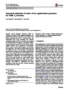
where ξi is the standard Gaussian random variable, and ε refers to the relative noise level. The variance σ02 is related to the noise level ε by σ0 = max1≤i≤100 {|yi |}ε. The parameter α is taken to be α = 1. The automatically determined value of the regularization parameter η depends on the realization of the random noise, and thus it is also random. The probability density p(η) is estimated from 1000 samples with kernel density estimation technique in a logarithmic scale [19] for Example 1, and it is shown in 15

10

20

8 7

8

15

6 5 p(σ2)

p(e)

p(η)

6 10

4

4

3 5

2

2 1

(a)

0 −10 10

−8

10

−6

10

−4

10

η

−2

10

0 −3 10

0

10

(b)

−2

−1

10

0

10 e

1

10

10

0 −10

(c) 10

−8

10

−6

10

−4

σ2

10

−2

10

0

10

Figure 1: Density of (a) η, (b) e, and (c) σ 2 for Example 1. Table 2: Numerical results for Example 1. ε 5e-6 5e-5 5e-4 5e-3 5e-2

σ02 3.34e-10 3.31e-8 3.31e-6 3.31e-4 3.31e-2

2 σGCV 2.48e-10 2.51e-8 2.52e-6 2.54e-4 2.52e-2

2 σGT 3.24e-10 2.60e-8 3.20e-6 2.72e-4 2.99e-2

ηQO 2.87e-8 9.87e-6 3.68e-5 1.08e-2 1.02e-2

ηLC 5.81e-10 6.27e-8 3.02e-6 1.53e-4 7.44e-3

ηGCV 2.30e-8 9.97e-7 1.70e-5 4.58e-4 1.16e-2

ηGT 4.74e-7 8.83e-6 2.20e-4 4.34e-3 1.08e-1

λGT 1.01e0 1.01e0 1.01e0 1.03e0 1.13e0

eQO 3.26e-2 4.55e-2 5.33e-2 1.52e-1 1.60e-1

eLC 3.67e-2 5.60e-2 9.38e-2 7.48e-2 1.58e-1

eGCV 3.28e-2 4.09e-2 5.86e-2 8.02e-2 1.61e-1

eGT 3.32e-2 4.53e-2 5.80e-2 1.35e-1 1.88e-1

Figure 1(a). Here the dash-dotted, dotted, dashed and solid curves refer to results given by ηQO , ηLC , ηGCV and ηGT , respectively. For medium noise levels, all three methods except the GCV work very well, however the variation of ηQO and ηLC are larger than that of ηGT . The GCV fails for about 10% of the samples, signified by ηGCV taking very small values, e.g. 1 × 10−20 . This phenomenon occurs irrespective of noise levels, and it is attributed to the fact that the GCV curve is very flat [16], see e.g. Figure 2(c). On average, ηLC decays to zero faster than ηQO and ηGT as the noise level σ02 tends to zero. Thus for low noise levels, ηLC often takes very small values and spans over a broad scale, which renders its solution plagued with spurious oscillations, see e.g. the red dotted curve in Figure 1(b). The observation concurs with previous theoretical and numerical results of Hanke [14] that suggest the L-curve criterion may suffer from nonconvergence in case of smooth solutions. The quasi-optimality criterion fails also occasionally, as indicated by the long tail, despite its overall robustness. Therefore, the newly proposed choice rule is more robust than the other three. The inverse solution xη∗ is also random. We utilize the accuracy error e defined below as the error metric e = kxη∗ − xkL2 . The probability density p(e) of the accuracy error e is shown in Figure 1(b). The accuracy errors eQO and eGT are very similar despite the apparent discrepancies of the regularization parameters, whereas eLC and eGCV vary very broadly, especially at low noise levels, although the variation of eLC is much 2 2 milder than that of eGCV . The estimates σGCV and σAT are practically identical, see Figure 1(c), which 2 2 qualifies σGT as an estimator of the variance. Interestingly, σGCV can slightly under-estimate the noise 2 2 level σ0 compared σGT due to the exceedingly small regularization parameters chosen by the GCV. 4

10

2

10

−1

2.5

σ2 λ η e

2

10 exact numerical

−2

10

0

G(η)

1.5 x

10

−2

10

1

−3

10 −4

10

0.5

−6

10

(a)

0

5

10 k

15

20

(b)

0 −2 −1.5 −1 −0.5

−4

0 t

0.5

1

1.5

2

10

−15

(c)10

−10

10

−5

10 η

0

10

5

10

Figure 2: (a) convergence of σ 2 , λ, η and e, (b) solution, and (c) GCV curve for Example 1 with ε = 5%.

16

10

8

8

8

6

6

p(σ2)

p(e)

p(η)

6 4

4

4 2

2

(a)

0 −10 10

−8

10

−6

10 η

−4

10

−2

10

0

2

−4

(b) 10

−3

10

−2

10 e

−1

10

0

10

0 −10

(c) 10

−8

10

−6

10

−4

σ2

10

−2

10

0

10

Figure 3: Density of (a) η, (b) e, and (c) σ 2 for Example 2. Next we investigate the convergence of Algorithm I for a particular realization of the noise. The numerical results are summarized in Figure 2 and Table 2. The algorithm converges within five iterations, and thus it merits a fast convergence. Moreover, the convergence is rather steady, and a few extra iterations would not deteriorate the inverse solution. The estimate σ 2 (η) changes very little during the iteration process, and a striking convergence within one iteration is observed, concurring with previous numerical findings for severely ill-posed problems [19]. The convergence of the estimate σ 2 (η) is mono2 tonic, substantiating the remark after Theorem 4.1. The estimate σGCV also approximates reasonably 2 2 σ0 , but it is less accurate than σGT , see Table 2. The prefactor λ remains almost unchanged as the 2(1−d)

noise level varies, see Table 2, and thus ηGT is indeed proportional to φ(x, y δ )1−d ≈ σ0 numerical solution remains accurate and stable for up to ε = 5%, see Figure 2(b).

5.2

4

= σ03 . The

Case 2: L2 -H 2 with constraint

Example 2. (1D gravity surveying [17] with nonnegativity constraint). The functions k and x are given ¡1 ¢− 3 by k(s, t) = 41 16 + (s − t)2 2 and x(t) = sin(πt) + 12 sin(2πt), respectively, and the integration interval is [0, 1]. The constrained optimization problems are solved by built-in MATLAB function quadprog. The presence of the constraint rules out the usage of the quasi-optimality criterion and the GCV, and it can also distort the shape of the L-curve greatly so that a corner does not appear at all, e.g. in case of the L2 -L2 functional. There does exist a distinct corner on the curve for the L2 -H 2 functional, see Figure 4(c), however, it is numerically difficult to locate due to the lack of monotonicity and discrete nature of sampling points. This causes the frequent failure of the MATLAB functions corner and l corner provided by the package, and visual inspection is required. The inconvenience persists for the remaining examples, and thus we do not investigate its statistical performance via computing relevant probability densities. The results for the L-curve criterion are obtained by manually locating the corner. However, the presence of constraints poses no difficulty to the proposed rule. Analogous to Example 1, ηGT and eGT are narrowly distributed, see Figures 3(a) and (b), which clearly illustrates its excellent 2 scalability with respect to the noise level. The estimate σGT peaks around the exact variance σ02 , and always retains the correct magnitude, see Figure 3(c). Typical numerical results for Example 2 with ε = 5% are presented in Figure 4. A fast and steady convergence of the algorithm within five iterations is again observed, see Figure 4(a), and similar convergence behavior is observed for other noise levels. In contrast, in order that the L-curve is representative, many points on the curve must be sampled, which effectively diminishes its computational efficiency. The numerical solution is in good agreement with the exact one, see Figure 4(b) and Table 3. The accuracy error eGT improves steadily as the noise level ε decreases, and it compares very favorably with eLC , for which a nonconvergence phenomenon is observed. The prefactor λ changes very little as the noise level ε varies, and thus ηGT decays at a rate commensurate 4 3 , see also Figure 3(a). with σGT

17

ε 5e-6 5e-5 5e-4 5e-3 5e-2

σ02 1.14e-9 1.14e-7 1.14e-5 1.14e-3 1.14e-1

Table 3: Numerical results for Example 2. 2 σGT ηLC ηGT λGT eLC 8.62e-10 7.20e-12 3.72e-10 4.11e-4 1.71e-1 8.67e-8 7.91e-11 8.06e-9 4.12e-4 1.11e-1 8.57e-6 9.54e-9 1.74e-7 4.15e-4 6.86e-2 8.58e-4 5.18e-7 3.81e-6 4.24e-4 1.65e-2 8.69e-2 6.25e-5 1.04e-4 5.32e-4 1.10e-1

0

10

eGT 4.84e-4 7.83e-4 2.49e-2 7.20e-3 4.12e-2

8

1.4

10 exact numerical

1.2 −2

10

1

x

10

0.6

σ2 λ η e

−6

10

0

0

5

10 k

10

0.4 0.2

−8

(a)

||Lx||2L2

−4

10

4

10

0.8

15

20

(b)

0 0

−4

0.2

0.4

0.6

0.8

10

1

−2

−1

(c) 10

t

10

0

||Kx−y||2L2

1

10

10

Figure 4: (a) convergence of σ 2 , λ, η and e, (b) solution, and (c) L-curve for Example 2 with ε = 5%.

5.3

Case 3: L2 -T V

Example 3 (numerical differentiation, adapted from deriv2 [16]). The functions k and x are given by ½ ½ s(t − 1), s < t, 1, 13 < t ≤ 23 , k(s, t) = and x(t) = t(s − 1), s ≥ t, 0, otherwise, respectively, and the integration interval is [0, 1]. The constant α is taken to be 5 × 10−3 , and η0 is 1 × 10−6 . The exact solution x is piecewise constant, and thus T V regularization is suitable. The regularization parameter ηGT distributes narrowly, and the accuracy error eGT is mostly comparable with the noise level, see Figures 5(a) and (b), respectively. The sample mean of the estimate 2 σGT (η) agrees excellently with the exact one σ02 , see Figure 5(c). For instance, in case of ε = 5%, the mean 1.23 × 10−5 almost coincides with the exact value. Typical numerical results for Example 3 are summarized in Figure 6 and Table 4. The L-curve has only an ambiguous corner, and the ambiguity persists for very low noise levels, e.g. ε = 5 × 10−6 . Nevertheless, the regularization parameters chosen by these two rules are comparable, and the numerical results are practically identical, see Table 4. Algorithm I converges within less than five iterations with an empirical asymptotic convergence rate r∗ < 0.15 for all five noise levels, and moreover it tends to accelerate as σ02 decreases, e.g. r∗ ≈ 0.05 for ε = 5 × 10−6 . Therefore, the algorithm is computationally very efficient. The reconstructed profile remains accurate and stable for ε up to 5%, see Figure 6(b) and Table 4. Note that it exhibits typical

10

8

8

8

6

6

p(σ2)

p(e)

p(η)

6 4

4

4 2

2

0 −10

(a) 10

−8

10

−6

10 η

−4

10

−2

10

0

2

−4

(b) 10

−3

10

−2

10 e

−1

10

0

10

0 −14

(c) 10

−12

10

Figure 5: Density of (a) η, (b) e and (c) σ 2 for Example 3. 18

−10

10

−8

σ2

10

−6

10

−4

10

ε 5e-6 5e-5 5e-4 5e-3 5e-2

σ02 1.19e-13 1.19e-11 1.19e-9 1.19e-7 1.19e-5

Table 4: Numerical results for Example 3. 2 σGT ηLC ηGT λGT eLC 8.21e-14 6.43e-12 4.70e-10 2.49e-1 1.26e-3 8.79e-12 3.59e-9 1.06e-8 2.49e-1 5.01e-3 8.65e-10 1.26e-7 2.25e-7 2.48e-1 4.34e-2 8.60e-8 2.01e-6 4.78e-6 2.45e-1 8.68e-2 8.89e-6 7.05e-5 1.08e-4 2.51e-1 1.05e-1

2

10

eGT 5.77e-4 9.38e-3 4.93e-2 8.08e-2 9.69e-2

4

1.2

10

1 0

10

0.8 exact numerical

x

10

0

10

0.6

|x|TV

σ2 λ η e

−2

0.4

−4

10

0.2

−4

10

0 −6

10

(a)

0

5

10 k

15

20

−0.2 0

(b)

−8

0.2

0.4

0.6

0.8

10 −10 10

1

−8

10

(c)

t

−6

||Kx−y||2L2

−4

10

10

Figure 6: (a) convergence of σ 2 , λ, η and e, and (b) solution, and (c) L-curve for Example 3 with ε = 5%. stair-cases of TV regularization.

5.4

Case 4: L2 -L1

£ ¤ Example 4 (Sparse reconstruction, adapted from Phillips’ problem [16]). Let φ(t) = 1 + cos πt 3 χ|t−s|