A New Method for Determining Optimal Regularization Parameter in

Hindawi Shock and Vibration Volume 2018, Article ID 7303294, 13 pages https://doi.org/10.1155/2018/7303294

Research Article A New Method for Determining Optimal Regularization Parameter in Near-Field Acoustic Holography Yue Xiao Jiangxi Province Key Laboratory of Precision Drive and Control, School of Mechanical and Electrical Engineering, Nanchang Institute of Technology, Nanchang, Jiangxi 330099, China Correspondence should be addressed to Yue Xiao; [email protected] Received 29 September 2017; Revised 17 January 2018; Accepted 24 January 2018; Published 20 February 2018 Academic Editor: Chao Tao Copyright © 2018 Yue Xiao. This is an open access article distributed under the Creative Commons Attribution License, which permits unrestricted use, distribution, and reproduction in any medium, provided the original work is properly cited. Tikhonov regularization method is effective in stabilizing reconstruction process of the near-field acoustic holography (NAH) based on the equivalent source method (ESM), and the selection of the optimal regularization parameter is a key problem that determines the regularization effect. In this work, a new method for determining the optimal regularization parameter is proposed. The transfer matrix relating the source strengths of the equivalent sources to the measured pressures on the hologram surface is augmented by adding a fictitious point source with zero strength. The minimization of the norm of this fictitious point source strength is as the criterion for choosing the optimal regularization parameter since the reconstructed value should tend to zero. The original inverse problem in calculating the source strengths is converted into a univariate optimization problem which is solved by a onedimensional search technique. Two numerical simulations with a point driven simply supported plate and a pulsating sphere are investigated to validate the performance of the proposed method by comparison with the L-curve method. The results demonstrate that the proposed method can determine the regularization parameter correctly and effectively for the reconstruction in NAH.

1. Introduction Near-field acoustic holography (NAH) is an effective technique for noise sources identification and acoustic field visualization. By measurements on a hologram surface near the sound source, the acoustic quantities such as pressure, particle velocity, and intensity anywhere including the source surface can be reconstructed, and the three-dimensional acoustic filed can be predicted. In the past years, many alternative methods of transform algorithm for realizing the NAH have been developed, for example, the spatial Fourier transform [1, 2], the boundary element method [3– 5], the Helmholtz equation least squares method [6, 7], the statistically optimized method [8, 9], and the equivalent source method (ESM) [10–14]. Among the methods, the ESM has attracted more attention with the advantages of the simple principle, the high calculation efficiency, and good adaptability for the shapes of the sound sources. However, the reconstruction of acoustic quantities of sound sources from near-field measurement data is an inverse problem, which is different from the traditional acoustic radiation calculation. Consequently, the reconstruction stability

is a key problem in NAH technology due to the fact that the realization process is ill-posed and the reconstructed results are highly sensitive to signal-to-noise ratio (SNR) [15]. If the conventional method for solving inverse matrix from the source to the hologram surface is used directly, the measurement error on the hologram surface as the input may be amplified sharply, and even the reconstructed results are completely unavailable. At present, the regularization approach has been widely used in the reconstruction process to restrict the influence of measurement errors on the reconstructed results and ensure the validity of the reconstruction performance. Currently, the direct regularization methods and the iterative regularization methods are mostly used for dealing with ill-posed problem of NAH [16, 17]. The direct regularization methods include truncated singular value decomposition (TSVD) method [18] and Tikhonov regularization method [19–21]. The iterative regularization methods include Landweber iterative regularization method [22] and conjugate gradient method [23]. The essence of the regularization method is to find an optimal approximate solution to the actual solution by a certain control strategy. So far there is no single regularization that is absolutely superior to the rest.

2

Shock and Vibration

For each of different regularization methods, the selection criteria of the optimal regularization parameters are the critical factors that determine the regularization effect. The methods for selection of optimal regularization parameter can be classified into prior [24] and posterior strategy. Compared with prior strategy, the posterior strategy does not require the prior knowledge of the noise variance in advance. The generalized cross validation (GCV) method [25] and the L-curve method [26, 27] as the posterior strategy are the two most widely used methods for selecting the optimal regularization parameters, both of which have good adaptability in the engineering application. Although the convergence of the GCV criterion has been proven theoretically, the GCV function curve sometimes is too flat, which makes it difficult to determine the minimum value of the GCV function. The L-curve method describes the comparison between the solution norm and residual norm with the regularization parameters in a log-log scale coordinate and adopts the maximum curvature of L-curve as the location of the optimal parameter. The L-curve method is reliable for determination of the optimal regularization parameter in most cases, but it may fail to search the maximum curvature position when there is more than one inflexion on the curve or the curve is not L-shaped approximately [28]. This paper focuses on a new method for determining the optimal parameters of Tikhonov regularization in NAH technique based on the ESM. In the proposed method, the transfer matrix from the source to the hologram surface is updated by augmenting a fictitious point source with zero strength near the locations of the equivalent sources. The minimization of the norm of this fictitious point source strength can be as the criterion for selection of the optimal regularization parameter since the reconstructed value should tend to zero. Thus the original inverse problem is converted into a univariate optimization problem that can be solved by one-dimensional search technique. The numerical simulations are investigated to demonstrate the validity of the proposed method, and the results show that the novel proposed method is able to select the regularization parameter correctly and effectively.

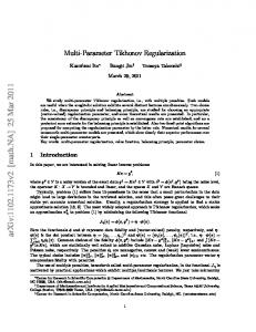
2. NAH Based on ESM The basic idea of the NAH based on ESM is that the actual radiated sound field can be replaced by superposing the acoustic field produced by a number of equivalent sources distributed inside the source surface. The source strengths of the equivalent sources can be evaluated by matching the acoustic pressures measured on the hologram surface, and the acoustic quantities in the acoustic field can be obtained by the source strengths and the transfer matrices constructed by the equivalent sources. As shown in Figure 1, the hologram surface Sh is placed near the outside of the source surface S, and the equivalent source surface Sq is located on the other side of the source surface S. Suppose that there are 𝑁 equivalent sources on the surface Sq , and the acoustic pressure at the field point r can be expressed as 𝑁

𝑝 (r) = ∑ i𝜌𝑐𝑘𝑔 (r, rq𝑛 ) 𝑞 (rq𝑛 ) , 𝑛=1

(1)

SＢ r − rＫn

r

S Sq

o

q(rＫn )

rＫn

z y

x

rＭl

rＭl − rＫn

rＢm

n

p(rＢm )

Figure 1: Schematic diagram of NAH based on ESM.

where 𝑝(r) is the acoustic pressure at the field point r, 𝜌 is the density of the medium, 𝑐 is the speed of sound, 𝑘 = 𝜔/𝑐 = 2𝜋/𝜆 is the wave number, 𝜆 is the wavelength, 𝜔 is the angular frequency, rq𝑛 and 𝑞(rq𝑛 ) are the location vector and the strength of the 𝑛th equivalent source, respectively, and 𝑔(r, rq𝑛 ) is the free field Green’s function obtained from the expression 󵄨 󵄨 exp (i𝑘 󵄨󵄨󵄨󵄨r − rq𝑛 󵄨󵄨󵄨󵄨) (2) 𝑔 (r, rq𝑛 ) = 󵄨 󵄨 . 4𝜋 󵄨󵄨󵄨󵄨r − rq𝑛 󵄨󵄨󵄨󵄨 Given that 𝑀 measurement points (rh1 , rh2 , . . . , rh𝑀) are selected on the hologram surface Sh and by applying (1) to each point, the pressure column vector at the measurement positions can be represented in matrix form as Ph = Gh Q,

(3)

where Ph = [𝑝(rh1 ), 𝑝(rh2 ), . . . , 𝑝(rh𝑀)]T is the pressure column vector at 𝑀 measurement points on the hologram surface, Q = [𝑞(rq1 ), 𝑞(rq2 ), . . . , 𝑞(rq𝑁)]T is the source strength column vector of the equivalent sources, Gh (𝑚, 𝑛) = i𝜌𝑐𝑘𝑔(rh𝑚 , rq𝑛 ) is the transfer matrix relating the source strengths of the equivalent sources on the surface Sq to the measured pressures on the surface Sh , and rh𝑚 is the location vector of the mth measurement point on the hologram surface Sh . If the number of measurement points is not less than the number of equivalent sources, that is, 𝑀 ≥ 𝑁, the source strength column vector Q can be uniquely obtained by solving inverse of Gh as −1

H Q = G+h Ph = (GH h Gh ) Gh Ph ,

(4)

where the superscript “+” denotes the generalized inverse.

Shock and Vibration

3

By using the source strength column vector Q, the pressure and particle velocity on any field point r can be calculated as

is to suppress the oscillation of the solution and make the solution as smooth as possible. The normal equation associated with (9) is given by

𝑝 (r) = Gfp Q,

(𝛼) (GH = GH h Gh + 𝛼Ι) Q h Ph ,

(5)

V (r) = Gf v Q,

where Gfp and Gf v are the transfer matrices relating the source strengths of the equivalent sources on the surface Sq to the pressure and particle velocity at the field point r, respectively, and Gfp = [i𝜌𝑐𝑘𝑔 (r, rq1 ) , i𝜌𝑐𝑘𝑔 (r, rq2 ) , . . . , i𝜌𝑐𝑘𝑔 (r, rq𝑁)] , 𝜕𝑔 (r, rq1 ) 𝜕𝑔 (r, rq2 ) 𝜕𝑔 (r, rq𝑁) Gf v = [ , ,..., ]. 𝜕r 𝜕r 𝜕r

(6)

Similarly, the pressure and normal velocity on the surface of the acoustic source can be reconstructed in the matrix form as Ps = Gsp Q,

(7)

Vns = Gsv Q,

where Gsp and Gsv are the transfer matrices relating the source strengths of the equivalent sources on the surface Sq to the pressure and normal velocity on the surface of the source, respectively, and Gsp (𝑙, 𝑛) = i𝜌𝑐𝑘𝑔 (rs𝑙 , rq𝑛 ) , Gsv (𝑙, 𝑛) =

𝜕𝑔 (rs𝑙 , rq𝑛 ) 𝜕n

(8) ,

in which rs𝑙 is the location vector of the lth point on the surface of the source and n is the outward normal of the source surface S.

3. Tikhonov Regularization In practice, there always exist errors in the measured pressures on the hologram surface. If (4) is used to calculate the source strengths of the equivalent sources Q directly, the reconstructed results are not reliable. So it is very critical to take measures in stabilizing the reconstruction procedure. Now the Tikhonov regularization is one of the most effective and popular methods to deal with the inverse problem. This method transfers the solution of (3) into the minimization problem as Q(𝛼) = arg min 𝑄

󵄩2 󵄩 (󵄩󵄩󵄩Gh Q − Ph 󵄩󵄩󵄩2 + 𝛼 ‖Q‖22 ) ,

(9)

where 𝛼 > 0 is the regularization parameter, which controls the weight between the residual norm and the solution norm. The first term of the right side is used to make the approximate solution satisfy (3) as far as possible but cannot be strictly true, because the measured errors in Ph will cause the solution to deviate from the true value in the form of the oscillation with high frequency. The role of the second term

(10)

where Ι is the identity matrix. The Tikhonov regularization solution can be expressed as −1

H Q(𝛼) = (GH h Gh + 𝛼Ι) Gh Ph .

(11)

The regularization parameter 𝛼 determines the compromise between the residual norm ‖Gh Q − Ph ‖22 and the solution norm ‖Q‖22 , and it plays an indispensable role in designing stable inversion algorithms and in obtaining physically plausible solutions. More precisely, when 𝛼 is too large, the residual norm becomes huge, since the solution is overly smooth, which often leads to undesirable effects. Conversely, it may be unstable and plagued with spurious and nonphysical details when 𝛼 is too small. Therefore, the determination of the optimal regularization parameter constitutes one of the major inconveniences and difficulties in applying existing regularization method to NAH technique.

4. Method for Determining Optimal Regularization Parameter Many researchers have developed a number of selection criteria and algorithms from different points of view, and each of them has their merit, shortcoming, and applicable condition [29]. Most of the methods endeavor to excavate the prior knowledge of the original problem or set some assumptions to derive some criteria for determining the regularization parameters. Mathematically, the regularization solution is expected to be located in the neighborhood of the true solution, but in fact the current criteria are usually focused on the information of outputs, and the neighborhood is out of the question due to the absence of information of the true solution. For the reconstruction problem in NAH based on ESM, the following gives a new criterion, which can make use of the true solution information and has a clear physical meaning. After determining the positions of all the equivalent sources, the corresponding source strengths will be obtained by matching the acoustic pressures measured on the hologram surface. In this case, there is no sound source or source strength is zero except for the positions of the equivalent sources. Here, the proposed method is to add a fictitious point source to the location where there is no equivalent source near the surface Sq ; then the transfer matrix can be reconstructed to obtain a new augmented transfer matrix. Thus, the source strength column vector of the equivalent sources Q can be expressed as Q = [QT1 QT2 ]

T T

= [𝑞 (rq1 ) , 𝑞 (rq2 ) , . . . , 𝑞 (rq𝑁) , 𝑞 (rq𝑁+1 )]𝑁+1 ,

(12)

where Q1 and Q2 are the source strength column vector of the equivalent sources existing originally and the fictitious point source added later, respectively.

4

Shock and Vibration

Accordingly, the augmented transfer matrix can be written as

Gh = [Gh1

𝑔 (rh1 , rq1 ) 𝑔 (rh1 , rq2 ) [ [ 𝑔 (rh2 , rq1 ) 𝑔 (rh2 , rq2 ) [ Gh2 ] = i𝜌𝑐𝑘 [ [ .. .. [ . . [ [ 𝑔 (rh𝑀, rq1 ) 𝑔 (rh𝑀, rq2 )

Substituting (12) and (13) into (10), it can be transformed as H H (GH h1 Gh1 + 𝛼Ι1 ) Q1 + Gh1 Gh2 Q2 = Gh1 Ph , H H GH h2 Gh1 Q1 + (Gh2 Gh2 + 𝛼Ι2 ) Q2 = Gh2 Ph .

(14)

From (14), the unknown source strength of the fictitious point source can be obtained. Furthermore, the true value of Q2 is known (zero), which provides available information for the solution of the problem; that is, a good regularization solution for the updated augmented system corresponding to the part of the fictitious point source Q(𝛼) 2 should tend to zero. Therefore, the minimization of the norm of this fictitious source strength Q(𝛼) 2 can be the criterion for selection of the optimal regularization parameter: 𝛼opt = arg min 𝛼 s.t.

󵄩󵄩 󵄩󵄩 󵄩󵄩Q2 󵄩󵄩2 H (GH h Gh + 𝛼Ι) Q = Gh Ph .

(15)

Qualitatively, the change trend of the norm of strength of the fictitious source ‖Q2 ‖2 with the increase of regularization parameter 𝛼 can be deduced as follows: (a) When 𝛼 = 0, regularization does not work, and ‖Q2 ‖2 is much larger than its true value (true value of ‖Q2 ‖2 is zero) because it is contaminated by the measurement errors. (b) With the increase of 𝛼, the regularization starts to work and ‖Q2 ‖2 tends to its true value gradually. In this process, ‖Q2 ‖2 decreases with the increase of 𝛼; that is, ‖Q2 ‖2 goes from the large oscillation to its true value, which is zero. (c) With the decrease of ‖Q2 ‖2 , when ‖Q2 ‖2 reaches the point where the position is closest to the true value, it starts to deviate from its true value as 𝛼 gradually increases. So in this process, ‖Q2 ‖2 increases with the increase of 𝛼. (d) Note that the norm of strengths of the equivalent sources ‖Q‖2 decreases monotonically with 𝛼; that is, ‖Q‖2 → 0 as 𝛼 → ∞, and thus ‖Q2 ‖2 → 0. When ‖Q2 ‖2 increases to a certain level with 𝛼, it begins to tend to zero with the increase of 𝛼. When 𝛼 is too large, the solving process produces an overregularization with too large regularization error. Therefore, it can be seen that the optimal regularization parameter should be at the point corresponding to the first local minimum where ‖Q2 ‖2 goes from decreasing to increasing. The minimization problem related to (15) can be solved by one-dimensional search technique, which is exactly the same

⋅ ⋅ ⋅ 𝑔 (rh1 , rq𝑁) 󵄨󵄨󵄨󵄨 𝑔 (rh1 , rq𝑁+1 ) 󵄨󵄨 󵄨 ⋅ ⋅ ⋅ 𝑔 (rh2 , rq𝑁) 󵄨󵄨󵄨 𝑔 (rh2 , rq𝑁+1 ) 󵄨󵄨 󵄨󵄨 .. .. 󵄨󵄨 󵄨󵄨 d . . 󵄨󵄨 󵄨󵄨 ⋅ ⋅ ⋅ 𝑔 (rh𝑀, rq𝑁) 󵄨󵄨󵄨 𝑔 (rh𝑀, rq𝑁+1 )

] ] ] ] ] ] ]

.

(13)

]𝑀×(𝑁+1)

as the L-curve method in the Matlab package developed by Hansen [30]. In order to capture the optimal solution more easily in the search interval, the logarithmic scale coordinate is also used to ensure that the curve of ‖Q2 ‖2 with 𝛼 can be flat and broad in the vicinity of the optimal solution. Furthermore, considering the initial situation without the fictitious point source, the corresponding solution equation can be expressed as H (GH h1 Gh1 + 𝛼Ι1 ) Q1 = Gh1 Ph .

(16)

According to (14), if Q2 ≠ 0, Q1 will contain the additional interference generated by Q2 . In order to obtain a better solution, after determining the optimal regularization parameter 𝛼opt , (16) is used to solve for Q1 as the final solution, which can be expressed as (𝛼

)

H Q1 opt = (GH h1 Gh1 + 𝛼opt Ι1 ) Gh1 Ph .

(17)

Thus, by using the reconstructed source strength column (𝛼 ) vector Q1 opt , the acoustic quantities anywhere in the sound field can be predicted. In addition, the essence of the proposed method to select the regularization parameter can be illustrated by the physical process of the equivalent source method. If the original 𝑁 equivalent sources can match the sound pressure on the hologram surface properly, then a good approximation for the sound field can be obtained by using the 𝑁 equivalent sources. To date, many literatures have been published and several satisfactory results have been obtained for setting the appropriate 𝑁. In general, if the number of measurement points is greater than the number of equivalent sources (𝑁 ≤ 𝑀), the strengths of the 𝑁 equivalent sources can be uniquely determined by the singular value decomposition (SVD) technique. Thus the sound field can be replaced directly by using the 𝑁 equivalent sources, and the source strength column vector of the original equivalent sources can be obtained by using (10) as −1

H Q1 = (GH h1 Gh1 + 𝛼Ι1 ) Gh1 Ph ,

(18)

where Q1 is the source strength column vector of the original equivalent sources before the fictitious source is added.

Shock and Vibration

5 102

102

 = 3.7901e − 3

101

 = 1.1933e − 2 ‖Q‖2

‖Q‖2

101

100

100

10−1

10−1

10−2 10−2

10−1

  GＢ Q − PＢ 2

100

(a)

10−2 10−2

10−1   GＢ Q − PＢ 2

100

(b)

Figure 2: L-Curve of the pressure reconstruction for the vibrating plate at (a) 500 Hz and (b) 800 Hz.

When 𝑁 + 1 equivalent sources are used to approximate the sound field and the positions of 𝑁 equivalent sources are unchanged, Q1 can be obtained by using (14) as −1

H H Q1 = (GH h1 Gh1 + 𝛼Ι1 ) (Gh1 Ph − Gh1 Gh2 Q2 ) .

(19)

By comparing (18) with (19), it is possible to obtain −1

H (Q1 − Q1 ) = (GH h1 Gh1 + 𝛼Ι1 ) (Gh1 Gh2 Q2 ) .

(20)

According to the properties of 2-norm, there is an inequality as 󵄩 󵄩󵄩 −1 H 󵄩󵄩 󵄩 󵄩 󵄩󵄩Q1 − Q1 󵄩󵄩󵄩 = 󵄩󵄩󵄩󵄩(GH 󵄩 󵄩2 󵄩 h1 Gh1 + 𝛼Ι1 ) Gh1 Gh2 Q2 󵄩󵄩󵄩2 󵄩󵄩 −1 󵄩 󵄩󵄩 󵄩 󵄩 󵄩 ≤ 󵄩󵄩󵄩(GH G + 𝛼Ι1 ) 󵄩󵄩󵄩 ⋅ 󵄩󵄩󵄩󵄩GH h1 Gh2 󵄩 󵄩2 󵄩 h1 h1 󵄩2 󵄩󵄩 󵄩󵄩 ⋅ 󵄩󵄩Q2 󵄩󵄩2 (21) = cond (GH h1 Gh1 + 𝛼Ι1 ) 󵄩 󵄩󵄩 H 󵄩󵄩Gh1 Gh2 󵄩󵄩󵄩 󵄩 󵄩 󵄩2 󵄩 ⋅ 󵄩󵄩 H 󵄩 ⋅ 󵄩󵄩Q2 󵄩󵄩 , 󵄩󵄩Gh1 Gh1 + 𝛼Ι1 󵄩󵄩󵄩2 󵄩 󵄩2 −1 H H where cond(GH h1 Gh1 + 𝛼Ι1 ) = ‖(Gh1 Gh1 + 𝛼Ι1 ) ‖2 ⋅ ‖Gh1 Gh1 + H 𝛼Ι1 ‖2 is the condition number of (Gh1 Gh1 + 𝛼Ι1 ). From (21), it is obvious that if ‖Q2 ‖2 → 0, then ‖Q1 − T Q1 ‖2 → 0; that is, Q1 → Q1 . Thus [Q1 0]T can be regarded as a good special solution to approximate the sound field when using 𝑁 + 1 equivalent sources. That is, constructing such a good special solution of the 𝑁 + 1 dimensional source strengths can be a suitable criterion to determine the optimal regularization parameter. When this criterion is satisfied, a good regularization parameter can be determined because the sound field can be approximated using the 𝑁 + 1 equivalent sources (the source strengths column vector is T [Q1 0]T ) and using N equivalent sources.

5. Numerical Simulations To examine the performance of the proposed method to determine the optimal regularization parameter in NAH, two numerical simulations were investigated, and the reconstruction results by using the proposed method were compared with those by using the L-curve method. 5.1. Simulation 1: A Vibrating Plate. This simulation case is a point driven simply supported aluminum plate with the thickness of 3 mm mounted in an infinite baffle. The dimension of the plate is 0.3 m × 0.3 m, and a harmonic force with an amplitude of 1 N is exerted vertically to the plate at the center. The radiated sound field is calculated by using Rayleigh’s integral formulation [31]. The center of the plate is set as the coordinate origin, and the 𝑥-axis and 𝑦-axis are parallel to the edges of the plate, respectively. The hologram plane and the equivalent source plane are placed at z = 0.05 m and 𝑧 = −0.03 m, respectively, with the same dimension as the plate and a measurement gird of 25 × 25. The random noise is added to the measurement data at a level of 30 dB. A fictitious point source with zero strength is located at 0 m, 0 m, and −0.03 m. The pressure and normal surface velocity on a plane 0.03 m away from the plate (z = 0.03 m) were reconstructed based on the “measured” pressures on the hologram surface, and the L-curve method and the proposed method are used to determine the optimal parameters of Tikhonov regularization. To quantify the reconstruction accuracy, the relative error is defined in the percentage form as 󵄩 󵄩󵄩 󵄩󵄩Are − Ath 󵄩󵄩󵄩2 × 100%, (22) 𝐸= 󵄩󵄩 󵄩󵄩 󵄩󵄩Ath 󵄩󵄩2 where Are is the reconstructed pressure or normal surface velocity and Ath is the corresponding theoretical value. Figure 2 shows the L-curves of the pressure reconstruction for the vibrating plate using the Matlab package developed by Hansen at 500 Hz and 800 Hz. The values of

6

Shock and Vibration 0.06

0.05

0.04

  Q2 2

  Q2 2

0.04 0.03

0.02 0.02

0 10−3

10−2

10−1

100

0.01 10−3

10−2

10−1

 ＩＪＮ  determined by the L-curve method (a)

100

 ＩＪＮ  determined by the L-curve method (b)

Figure 3: Object function versus the regularization parameter of the pressure reconstruction for the vibrating plate at (a) 500 Hz and (b) 800 Hz.

regularization parameter are determined as 1.1933 × 10−2 and 3.7901 × 10−3 at the corner of the L-curve, respectively, and the relative errors between the reconstructed pressure and the theoretical value are 6.68% and 6.37% by using the parameters for regularization, respectively. Figure 3 shows the change curve of the object function ‖Q2 ‖2 with the regularization parameter 𝛼 by using the proposed method at 500 Hz and 800 Hz. The trends of the curves are consistent with the speculation mentioned above. The regularization parameters can be chosen as 1.0010 × 10−2 and 3.5481 × 10−3 at the minimum of the curve, and the relative errors are 6.63% and 6.44%, respectively. For comparison, the locations of the parameter determined by using the Lcurve method are also marked in Figure 3. It can be found that the values of the regularization parameter determined by using the L-curve method and the proposed method are very close, and both methods can give an appropriate regularization parameter for the pressure reconstruction in NAH. In addition, as shown in Figure 3, if a linear scale is used for searching the regularization parameter, the optimal solution may be crossed in the very narrow V-shaped region containing it and stray into the right side of the monotonically decreasing interval, which will result in a search failure. In the proposed method, the logarithmic scale is used to extend the search interval of regularization parameter, so it is easier to search for the optimal solution. Figure 4 presents the comparisons of the reconstructed pressure with the corresponding theoretical value by using the two methods at 500 Hz and 800 Hz. It can be seen that the reconstructed results by using these two methods show good agreements with the theoretical values. The L-curve of the pressure reconstruction for the vibrating plate at 1000 Hz is shown in Figure 5. It can be seen that there is more than one inflexion on the L-curve, which causes the L-curve method to have a wrong detection for the regularization parameter.

The regularization parameter is determined as 6.9374, and the reconstruction error is 53.46%. As a comparison, Figure 6 shows the curve of the proposed method for choosing the regularization parameter. The regularization parameter by using the proposed method is 2.1877 × 10−3 , and the reconstructed relative error is 6.68%, which is much smaller than that by using the L-curve method. By the comparison of the two errors, it can be seen that the proposed method is valid for the pressure reconstruction when the L-curve method fails to determine the regularization parameter. The comparison of the reconstructed pressure with the corresponding theoretical value at 1000 Hz is shown in Figure 7. It can be seen that the reconstructed pressure by using the L-curve method differs largely from the theoretical value due to the overregularization, while the reconstructed pressure by using the proposed method can give a better reconstruction. Figure 8 shows the L-curve of the normal surface velocity reconstruction for choosing regularization parameter at 600 Hz. It can be seen that the position of the optimal parameter is not located at the corner of the L-curve, and there is a wrong detection problem in the L-curve method. The regularization parameter is determined as 233.27, which seems too large. Using the parameter determined by the Lcurve method for regularization, the reconstruction relative error is 43.68%. The curve of the proposed method used to determine the optimal regularization parameter is shown in Figure 9. The regularization parameter can be determined as 7.7618 × 10−2 by detecting the minimum of the curve. The relative error of the normal surface velocity in the proposed method is 5.97%, which is much smaller than that in the Lcurve method. Figure 10 shows the comparison of the amplitude distributions of the reconstructed normal surface velocities with the corresponding theoretical values by using the two methods at 600 Hz. It can be seen that there is overregularization in

Shock and Vibration

7

0.25

0.2

0.2

0.15

0

0.15

0.1

0.15

0 x (m)

(a)

0.05

−0.15 −0.15

0.15

0

(Pa)

(c)

(Pa)

0.15 0.3 0.2

0

0.2

0.1 0 x (m)

(Pa)

0.15

0.3

0.3 y (m)

0

0.15

x (m)

(b)

0.15

y (m)

0.15 0.1

0.05

−0.15 −0.15

x (m)

−0.15 −0.15

0.2 0

0.1

0.05 0

0.25

y (m)

−0.15 −0.15

(Pa)

0.15

0.25 y (m)

y (m)

0

(Pa)

0.15

y (m)

(Pa)

0.15

0

0.2 0.1

0.1 −0.15 −0.15

0.15

0 x (m)

(d)

−0.15 −0.15

0.15

0 x (m)

(e)

0.15

(f)

Figure 4: Comparison of reconstructed pressures. (a) Theoretical value at 500 Hz, (b) reconstructed by using the L-curve method at 500 Hz, (c) reconstructed by using the proposed method at 500 Hz, (d) theoretical value at 800 Hz, (e) reconstructed by using the L-curve method at 800 Hz, and (f) reconstructed by using the proposed method at 800 Hz.

103

2.5 2

  Q2 2

‖Q‖2

102

 = 6.9374

101

0 10−4

−1

10

1 0.5

100

10

1.5

−1

10

0

  GＢ Q − PＢ 2

10

1

10

2

Figure 5: L-Curve of the pressure reconstruction for the vibrating plate at 1000 Hz.

the L-curve method due to the fact that the optimal parameter determined by this method is too large, which results in losing too much information of the real holographic pressures. Meanwhile the reconstructed normal surface velocity by using the proposed method shows good agreement with the theoretical value, which indicates that the proposed method can choose a good regularization parameter when the Lcurve method has wrong detection. The influence of the position of the additional fictitious source on the reconstruction accuracy is also investigated to

10−3

10−2

10−1

100

101

 ＩＪＮ  determined by the L-curve method

Figure 6: Object function versus the regularization parameter of the pressure reconstruction for the vibrating plate at 1000 Hz.

validate the performance of the proposed method. Assume that the position of the additional fictitious point source moves along from −0.5 m to 0.5 m in z direction with an interval of 0.01 m, and that of x and y directions remains unchanged. The reconstruction relative errors for different positions of the additional fictitious source at 500 Hz are shown in Figure 11. It can be seen that the reconstruction errors are less than 7% except at the position of 𝑧 = 0.05 m (due to the fact that the position of the additional fictitious

8

Shock and Vibration (Pa)

0.15

5

2.5

3

0

2

0

1.5

0

0.5

−0.15 −0.15

0.15

3

0

2

1

1 −0.15 −0.15

5 4

2

y (m)

y (m)

4

(Pa)

0.15

y (m)

(Pa)

0.15

0

x (m) (a)

0.15

1 −0.15 −0.15

0

x (m)

x (m)

(b)

(c)

0.15

Figure 7: Comparison of reconstructed pressures at 1000 Hz. (a) Theoretical value, (b) reconstructed by using the L-curve method, and (c) reconstructed by using the proposed method.

1010

0.03

  Q2 2

‖Q‖2

0.02 105

0.01

 = 233.27

100

0 10−3

10−2

10−1

  GＢ Q − PＢ 2

100

101

Figure 8: L-Curve of the normal surface velocity reconstruction for the vibrating plate at 600 Hz.

point source coincides with the position of the measurement point on the hologram surface), which means that the proposed method is not sensitive to the position of the additional fictitious point source. Actually, as long as the position of the additional fictitious source is near the equivalent source surface, the proposed method can get a good regularization parameter to ensure stability of the reconstruction. 5.2. Simulation 2: A Pulsating Sphere. A pulsating sphere with a radius of 0.1 m is investigated as depicted in Figure 12. There are 62 nodes distributed on the source surface with the equal angle interval 𝜋/6. The analytical pressure of a pulsating sphere with a radius of 𝑎 at the point 𝑟 in the sound field can be expressed as 𝑝 (𝑟) =

𝑎 2𝜋𝑓𝜌𝑎 V exp [i𝑘 (𝑟 − 𝑎)] , 𝑟 0 i + 𝑘𝑟

(23)

where V0 is the radial velocity, 𝑎 is the sphere radius, and 𝑓 is the vibration frequency of sound source. In the simulation, the radial velocity V0 is 0.01 m/s, the air density 𝜌 is 1.2 kg/m3 , and the speed of sound 𝑐 is 344 m/s. The

10−2

10−1

100 

101

102

103

ＩＪＮ  determined by the L-curve method

Figure 9: Object function versus the regularization parameter of the normal surface velocity reconstruction for the vibrating plate at 600 Hz.

equivalent source surface is a spherical surface with a radius of 0.08 m and has the same distributed form as the source surface with 62 equivalent point sources. The hologram surface with the size of 1 m × 1 m is located 0.2 m away from the center of the sphere, and there are 16 × 16 measurement points distributed on the surface with a uniform interspacing. All the acoustic pressures on the hologram surface are given by (23). A fictitious point source with zero strength is located at 0.0739 m, 0.0173 m, and 0.040 m and the field point located at 0 m, 0 m, and 1 m is chosen as the reconstructed point. The random noise is added to the measurement data at a level of 30 dB. Figure 13 shows the L-curves of the pressure reconstruction for the pulsating sphere at 300 Hz, 500 Hz, 700 Hz, and 900 Hz. It can be seen that all the curves have a quite clear L-shape. The regularization parameters are determined as 1.0128 × 10−4 , 5.003 × 10−4 , 8.1372 × 10−4 , and 1.1166 × 10−3 at the corner of the L-curve, respectively, and the relative errors between the reconstructed pressure and the theoretical

Shock and Vibration

×10−3

×10−3

1.5 Normal surface velocity (m/s)

1.5 Normal surface velocity (m/s)

9

1 0.5 0 0.15

0.5 0 0.15

0.15

0

y(

1

m)

−0.15 −0.15

0.15

0 y( m)

0 )

x (m

−0.15

Normal surface velocity (m/s)

×10−3

1 0.5 0 0.15

0.15

0

m)

0 −0.15

Normal surface velocity (m/s)

1.5

y(

−0.15

)

x (m

(b)

(a)

1.5

0

1

0.5

0 −0.15

)

x (m

−0.15

×10

−3

0 x (m)

0.15

Theoretical value Reconstructed by using the L-curve method Reconstructed by using the proposed method (c)

(d)

Figure 10: Comparison of reconstructed normal surface velocities at 600 Hz. (a) Theoretical value, (b) reconstructed by using the L-curve method, (c) reconstructed by using the proposed method, and (d) normal surface velocity along the middle row. 100

80

60

40

z (m)

Relative error (%)

0.1

0

20

0 −0.5 −0.4 −0.3 −0.2 −0.1

0 0.1 z (m)

0.2

0.3

0.4

0.5

Figure 11: Reconstruction errors for different positions of the additional fictitious source at 500 Hz.

−0.1 0.1

0.1

)

value are 40.91%, 22.28%, 47.31%, and 58.59% by using the parameters for regularization, respectively.

0

0

y (m

−0.1 −0.1

m)

x(

Figure 12: The nodes distribution on the source surface of the pulsating sphere.

Shock and Vibration 1012

1012

109

109

106 10

 = 1.0128e − 4

‖Q‖2

‖Q‖2

10

3

100 10−3 10−2

106 10

100 10−1

  GＢ Q − PＢ 2

100

10−3 10−1

101

(a)

10

10

101

12

109  = 8.1372e − 4

‖Q‖2

‖Q‖2

109

103 100 10−3 10−1

100   GＢ Q − PＢ 2 (b)

12

106

 = 5.0031e − 4

3

106

 = 1.1166e − 3

103 100

100

  GＢ Q − PＢ 2

101

10−3 10−1

(c)

100   GＢ Q − PＢ 2

101

(d)

Figure 13: L-Curve of the pressure reconstruction for the pulsating sphere. (a) 300 Hz, (b) 500 Hz, (c) 700 Hz, and (d) 900 Hz.

By using the proposed method, the curves for choosing regularization parameter at 300 Hz, 500 Hz, 700 Hz, and 900 Hz are shown in Figure 14. The optimal regularization parameters are chosen as 2.7541 × 10−3 , 6.1662 × 10−3 , 1.3832 × 10−2 , and 2.6923 × 10−2 corresponding to the bottom of the curve, respectively, and the reconstruction relative errors are 9.89%, 3.22%, 11.86%, and 13.38%, respectively, all of which are much smaller than those by using the L-curve method. It can be seen that the proposed method can give a good regularization parameter in NAH technique based on the ESM. Figure 15 shows the relative errors between the reconstructed pressure and the theoretical value by using the two methods for choosing the regularization parameter over the frequency range from 50 Hz to 1000 Hz. It can be seen that the reconstruction errors by using the proposed method are always smaller than those determined by using the L-curve method, and the relative errors of pressure are below 20% over most of the whole frequency range, which demonstrates the validity of the proposed method for the selection of regularization parameter in NAH. The influence of the SNR on the reconstructed pressure at different frequencies is also examined. Figure 16 shows the reconstruction relative error versus SNR in the range of 10 dB to 50 dB by using the proposed method at 200 Hz, 300 Hz, 450 Hz, 600 Hz, 800 Hz, and 1000 Hz, respectively. It can be seen that the relative errors calculated by using proposed

method are insensitive to the change of SNR, which indicates that the proposed method is of good stability for choosing regularization parameter.

6. Conclusion A new optimal parameter selecting method for the Tikhonov regularization was proposed in NAH based on the ESM. In the proposed method, the criterion for determining the optimal regularization parameters was given by adding a fictitious point source with zero strength to make a part of the solution of the augmented problem known, which has a clear physical meaning. A one-dimensional search technique was used to minimize the norm of the fictitious point source strength for determination of the optimal parameter in the Tikhonov regularization method. The validity of the proposed method has been demonstrated by numerical simulations with kinds of sound sources including a point driven simply supported plate and a pulsating sphere. It was shown that the proposed method can get a better regularization parameter for the reconstruction with good accuracy and stability in NAH compared with the L-curve method. Future research will emphasize the existence and uniqueness of the minimum point on the curve of the norm of the fictitious point source strength with the regularization parameter in mathematics. The present work also can provide a new idea for solving other inverse problems, that is, try to add new known information

Shock and Vibration

11 0.9

0.8

0.6

  Q2 2

  Q2 2

0.6 0.4

0.3 0.2

0 10−4

10−3

10−2

10−1

0 10−4

101

100

10−3

10−2

10−1



100

101

100

101

 ＩＪＮ  determined by the L-curve method

ＩＪＮ  determined by the L-curve method (a)

(b)

0.9

0.6

0.6   Q2 2

  Q2 2

0.9

0.3

0.3

0 10−4

10−3

10−2

10−1

100

0 10−4

101

10−3

10−2

10−1



 ＩＪＮ  determined by the L-curve method

ＩＪＮ  determined by the L-curve method (c)

(d)

Figure 14: Object function versus the regularization parameter of the pressure reconstruction for the pulsating sphere at (a) 300 Hz, (b) 500 Hz, (c) 700 Hz, and (d) 900 Hz. 20

70

15

50

Relative error (%)

Relative error (%)

60

40 30 20

10

5

10 0 50

200

400

600

800

1000

0 10

20

The proposed method The L-curve method

Figure 15: Reconstruction errors of pressure by using the two methods versus frequency.

30

40

50

SNR (dB)

Frequency (Hz) 200 Hz 300 Hz 450 Hz

600 Hz 800 Hz 1000 Hz

Figure 16: Reconstruction errors of pressures by using the proposed method versus SNR.

12 to augment the transfer matrix and then make full use of the known information to constrain the solution to approximate the true value.

Shock and Vibration

[13]

Conflicts of Interest The authors declare that there are no conflicts of interest regarding the publication of this paper.

[14]

Acknowledgments

[15]

This work was supported by the Science and Technology Project of Education Department of Jiangxi Province (Grant no. GJJ151121) and the National Natural Science Foundation of China (Grant no. 51565037).

References [1] E. G. Williams, B. H. Houston, and P. C. Herdic, “Fast fourier transform and singular value decomposition formulations for patch nearfield acoustical holography,” The Journal of the Acoustical Society of America, vol. 114, no. 3, pp. 1322–1333, 2003. [2] D.-Y. Hu, C.-X. Bi, Y.-B. Zhang, and L. Geng, “Extension of planar nearfield acoustic holography for sound source identification in a noisy environment,” Journal of Sound and Vibration, vol. 333, no. 24, pp. 6395–6404, 2014. [3] I.-Y. Jeon and J.-G. Ih, “On the holographic reconstruction of vibroacoustic fields using equivalent sources and inverse boundary element method,” The Journal of the Acoustical Society of America, vol. 118, no. 6, pp. 3473–3482, 2005. [4] E. G. Williams, B. H. Houston, P. C. Herdic, S. T. Raveendra, and B. Gardner, “Interior near-field acoustical holography in flight,” The Journal of the Acoustical Society of America, vol. 108, no. 4, pp. 1451–1463, 2000. [5] H. B. Zhang, Q. Wan, W. K. Jiang, and C. J. Liao, “A study on holographic reconstruction of cyclostationary sound field based on boundary element method,” Journal of Vibration and Acoustics, vol. 132, no. 5, pp. 0545011–0545015, 2010. [6] S. F. Wu, M. Moondra, and R. Beniwal, “Analyzing panel acoustic contributions toward the sound field inside the passenger compartment of a full-size automobile,” The Journal of the Acoustical Society of America, vol. 137, no. 4, pp. 2101–2112, 2015. [7] S. F. Wu, The Helmholtz equation least squares method, Modern Acoustics and Signal Processing, Springer, New York, 2015. [8] Y. T. Cho, J. S. Bolton, and J. Hald, “Source visualization by using statistically optimized near-field acoustical holography in cylindrical coordinates,” The Journal of the Acoustical Society of America, vol. 118, no. 4, pp. 2355–2364, 2005. [9] C. Bi, X. Chen, J. Chen, and R. Zhou, “Nearfield acoustic holography based on the equivalent source method,” Science China Technological Sciences, vol. 48, no. 3, pp. 338–353, 2005. [10] J. Hald, “Basic theory and properties of statistically optimized near-field acoustical holography,” The Journal of the Acoustical Society of America, vol. 125, no. 4, pp. 2105–2120, 2009. [11] Y.-B. Zhang, F. Jacobsen, C.-X. Bi, and X.-Z. Chen, “Near field acoustic holography based on the equivalent source method and pressure-velocity transducers,” The Journal of the Acoustical Society of America, vol. 126, no. 3, pp. 1257–1263, 2009. [12] N. P. Valdivia, E. G. Williams, and P. C. Herdic, “Equivalent sources method for supersonic intensity of arbitrarily shaped

[16]

[17]

[18]

[19]

[20]

[21]

[22]

[23]

[24]

[25]

[26]

[27]

geometries,” Journal of Sound and Vibration, vol. 347, pp. 46– 62, 2015. Y. Xiao, J. Chen, D. Y. Hu, and F. X. Jiang, “Equivalent source method for identification of panel acoustic contribution in irregular enclosed sound field,” Chinese Journal of Acoustics, vol. 39, no. 1, pp. 49–66, 2015. C.-X. Bi, W.-Q. Jing, Y.-B. Zhang, and W.-L. Lin, “Reconstruction of the sound field above a reflecting plane using the equivalent source method,” Journal of Sound and Vibration, vol. 386, pp. 149–162, 2017. P.-A. Gauthier, A. G´erard, C. Camier, and A. Berry, “Acoustical inverse problems regularization: Direct definition of filter factors using signal-to-noise ratio,” Journal of Sound and Vibration, vol. 333, no. 3, pp. 761–773, 2014. S. Yoon and P. Nelson, “Estimation of acoustic source strength by inverse methods: part ii, experimental investigation of methods for choosing regularization parameters,” Journal of Sound and Vibration, vol. 233, no. 4, pp. 665–701, 2000. K. Chelliah, G. Raman, and R. T. Muehleisen, “An experimental comparison of various methods of nearfield acoustic holography,” Journal of Sound and Vibration, vol. 403, pp. 21–37, 2017. A. Sarkissian, “Method of superposition applied to patch nearfield acoustic holography,” The Journal of the Acoustical Society of America, vol. 118, no. 2, pp. 671–678, 2005. E. G. Williams, “Regularization methods for near-field acoustical holography,” The Journal of the Acoustical Society of America, vol. 110, no. 4, pp. 1976–1988, 2001. A. N. Thite and D. J. Thompson, “The quantification of structure-borne transmission paths by inverse methods. Part 2: Use of regularization techniques,” Journal of Sound and Vibration, vol. 264, no. 2, pp. 433–451, 2003. M. R. Bai and J.-H. Lin, “Source identification system based on the time-domain nearfield equivalence source imaging: Fundamental theory and implementation,” Journal of Sound and Vibration, vol. 307, no. 1-2, pp. 202–225, 2007. B.-K. Kim and J.-G. Ih, “Design of an optimal wave-vector filter for enhancing the resolution of reconstructed source field by near-field acoustical holography (NAH),” The Journal of the Acoustical Society of America, vol. 107, no. 6, pp. 3289–3297, 2000. N. P. Valdivia and E. G. Williams, “Study of the comparison of the methods of equivalent sources and boundary element methods for near-field acoustic holography,” The Journal of the Acoustical Society of America, vol. 120, no. 6, pp. 3694–3705, 2006. C. R. Vogel, Computational Methods for Inverse Problems, Society for Industrial and Applied Mathematics, Philadelphia, Pa, USA, 2002. H. G. Choi, A. N. Thite, and D. J. Thompson, “Comparison of methods for parameter selection in Tikhonov regularization with application to inverse force determination,” Journal of Sound and Vibration, vol. 304, no. 3–5, pp. 894–917, 2007. Q. Lecl`ere, “Acoustic imaging using under-determined inverse approaches: frequency limitations and optimal regularization,” Journal of Sound and Vibration, vol. 321, no. 3–5, pp. 605–619, 2009. K. Chelliah, G. G. Raman, and R. T. Muehleisen, “Enhanced nearfield acoustic holography for larger distances of reconstructions using fixed parameter Tikhonov regularization,” The Journal of the Acoustical Society of America, vol. 140, no. 1, pp. 114–120, 2016.

Shock and Vibration [28] Y. Zhang, C. Bi, L. Xu, and X. Chen, “Novel method for selection of regularization parameter in the near-field acoustic holography,” Chinese Journal of Mechanical Engineering, vol. 24, no. 2, pp. 285–292, 2011. [29] F. Bauer and M. A. Lukas, “Comparing parameter choice methods for regularization of ill-posed problems,” Mathematics and Computers in Simulation, vol. 81, no. 9, pp. 1795–1841, 2011. [30] P. C. Hansen, “Regularization tools: a Matlab package for analysis and solution of discrete ill-posed problems,” Numerical Algorithms, vol. 6, no. 1-2, pp. 1–35, 1994. [31] E. G. Williams, Fourier Acoustics: Sound Radiation and Nearfield Acoustical Holography, Academic Press, San Diego, CA, USA, 1999.

13

International Journal of

Rotating Machinery

(QJLQHHULQJ Journal of

Hindawi Publishing Corporation http://www.hindawi.com

Volume 201

The Scientific World Journal Hindawi Publishing Corporation http://www.hindawi.com

Volume 2014

International Journal of

Distributed Sensor Networks

Journal of

Sensors Hindawi Publishing Corporation http://www.hindawi.com

Volume 2014

Hindawi Publishing Corporation http://www.hindawi.com

Volume 2014

Hindawi Publishing Corporation http://www.hindawi.com

Volume 2014

Journal of

Control Science and Engineering

Advances in

Civil Engineering Hindawi Publishing Corporation http://www.hindawi.com

Hindawi Publishing Corporation http://www.hindawi.com

Volume 2014

Volume 2014

Submit your manuscripts at https://www.hindawi.com Journal of

Journal of

Electrical and Computer Engineering

Robotics Hindawi Publishing Corporation http://www.hindawi.com

Hindawi Publishing Corporation http://www.hindawi.com

Volume 2014

Volume 2014

VLSI Design Advances in OptoElectronics

International Journal of

Navigation and Observation Hindawi Publishing Corporation http://www.hindawi.com

Volume 2014

Hindawi Publishing Corporation http://www.hindawi.com

Hindawi Publishing Corporation http://www.hindawi.com

Chemical Engineering Hindawi Publishing Corporation http://www.hindawi.com

Volume 2014

Volume 2014

Active and Passive Electronic Components

Antennas and Propagation Hindawi Publishing Corporation http://www.hindawi.com

$HURVSDFH (QJLQHHULQJ

Hindawi Publishing Corporation http://www.hindawi.com

Volume 2014

+LQGDZL3XEOLVKLQJ&RUSRUDWLRQ KWWSZZZKLQGDZLFRP

9ROXPH

Volume 201-

International Journal of

International Journal of

,QWHUQDWLRQDO-RXUQDORI

Modelling & Simulation in Engineering

Volume 2014

Hindawi Publishing Corporation http://www.hindawi.com

Volume 2014

Shock and Vibration Hindawi Publishing Corporation http://www.hindawi.com

Volume 2014

Advances in

Acoustics and Vibration Hindawi Publishing Corporation http://www.hindawi.com

Volume 2014