a new decomposition-based pricing technique for solving large-scale

GANIT J. Bangladesh Math. Soc. (ISSN 1606-3694) 34 (2014) 5-20

A NEW DECOMPOSITION-BASED PRICING TECHNIQUE FOR SOLVING LARGE-SCALE MIXED IP WITH A COMPUTER TECHNIQUE A. Islam1, M. Babul Hasan2 and H. K. Das3 Department of Mathematics, Dhaka University of Engineering & Technology, Gazipur 2 Department of Mathematics, University of Dhaka, Dhaka-1000, Bangladesh 3 Department of Mathematics and Statistics, Concordia University, Montr´eal, Quebec, H3G 1M8, Canada E-mail: [email protected], [email protected], [email protected] 1

Received 24.07.2013

Accepted 07.12.2014

ABSTRACT In this paper, we develop a new Decomposition-Based Pricing (DBP) procedure to filter the unnecessary decision ingredients from large scale mixed integer programming (MIP) problem, where the variables are in huge number will be abated and the complicacy of restrictions will be straightforward. We then develop a generalized computer technique corresponding to our new DBP method by using the programming language A Mathematical Programming Language (AMPL). A number of examples have been illustrated to demonstrate our method.

Keywords: Lagrangian Dual, Sub-problem, Master-problem, Decomposition, DBP, Dual Pricing, MIP, AMPL 1. Introduction Management Science (MS), big Group of Companies and Industries or Government Policies (GP) are affiliated with a huge number of decision ingredients and complicated restrictions. Every factor in MS, every product in Industries and every decision in GP are not always bankable in practice. After formulating these models there arises large-scale LP. Thus more complication arises when some variables are bound to be integer which brings forth MIP problems. Thus, in decision science: production planning, refinery optimization, resource allocation, assignment, transportation, networking, TSP, game theory, after converting them into LPs and MIP, have computational bottleneck if for big companies do by such complicated situations. Almost five decades have passed since Ford and Fulkerson[5] suggested dealing only implicitly with the variables of a multi commodity flow problem. George Dantzig and Phil Wolfe[2] pioneered this fundamental idea, developing a strategy to extend a linear program column wise as needed in the solution process. This technique was first put to actual use by Gilmore and Gomory[9] as part of an efficient heuristic algorithm for solving the cutting-stock problem. Thus Dantzig-Wolf Decomposition (DWD) is nowadays a prominent method to cope with a huge number of variables but it has

6

Islam et al.

computational defects along with delayed column generation. It cannot be applied to solve structural dual inequalities, primal and dual stabilization strategies. Lagrangian was used by Held and Karp[13] based on minimum spanning trees for the traveling salesman problem, by Fisher[4] for scheduling problems and by Shapiro[21] for the general IP problem. Experience after Marshall L. Fisher[20], it is rare in practice that the Lagrangian solution will be feasible in the original problem. In the last decade, the new interiorpoint[6] algorithms and advanced implementations of simplex methods have been developed with impressive advances computer technology. Using it, we can now solve LPs with more than one million variables and thousands of constraints. It's not as intuitively satisfying because, these methods don't visit vertices. They wander through the interior region, converging on a solution when successful and take more time. In 2011, Md. Istiaq Hossain and M Babul Hasan[15] developed an Improved Decomposition Algorithm for solving large scale LPs depending on DWD principle. Also, in 2013 H. K. Das and Hasan[10] developed a primal dual approach of Linear fractional programming (LFP) and LP problem depending on DWD principle. But they did not mention the behavior of their algorithm in case of Large-Scale MIP. Actually large-scale problems are not easily partitioned in this way. The optimal solution is very sensitive to the overall variable interactions as working with a huge numbers of decision variables. The large-scale system approach is to treat the problem as a unit, devising specialized algorithms to exploit the structure of the problem. This alternative will be explored in this paper with the most important large-scale programming procedures by our new DBP. Mamer and McBride[16] developed DBP for multi-commodity flow problems earlier. In this paper, we propose an iterative partial pricing scheme for solving large-scale LPs and MIPs using the Simplex method. The approach solves a relaxed sub-problem to identify the nontrivial variables to be considered during the pricing step of the Simplex method. The goal of the procedure is to find an efficient set of candidate to enter the basis without incurring the cost of pricing of all the non-basic columns in the problem at the each iteration. Thus the trivial ingredients are filtered and constraints become simpler. Our scheme is motivated by the column-generation approach of DWD. The rest of the paper is organized as follows. In Section 2, we present some necessary definitions. In Section 3, we present some existing approaches to solve large-scale LPs. In Section 3, we present our new Decomposition-Based Pricing (DBP) technique with numerical examples and develop computer technique. Section 5 shows the comparative effectiveness of new DBP. The main objective of this work, the implementation of DBP procedure on MIP has been demonstrated in Section 6. 2. Preliminaries In this Section, we present some necessary definitions relevant to our purpose.

A New Decomposition-Based Pricing Technique for Solving

7

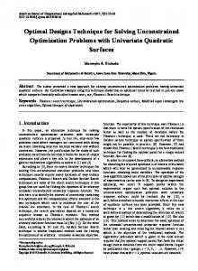
2.1. Polytope In elementary geometry, a polytope is a geometric object with flat sides, which exists in any general number of dimensions. A polygon is a polytope in two dimensions, a polyhedron in three dimensions, and so on in higher dimensions. A convex polytope may be defined as the convex hull of a finite set of points. An n-dimensional polytope may be specified as the set of solutions to a system of linear inequalities, Ax  b. Where A is a real s  n matrix and b is a real vector of dimension s.

Fig. 1: Polytop in various dimension

2.2. Lagrangian Dual concept To define Lagrangian Relaxation, we consider one combinatorial linear programming problem, P: Max{cx | Ax  b, Bx   X}. There are two types of constraint according to their structure. Now if, in case, we relax the first constraint then feasible region gets enhanced or remains the same. So, we define a conformable Lagrange Multiplier   0 and relax Ax  b. Then we get, PR: Max{cx +  (b – Ax) || Bx  d, x  X}. Here   0 and b – Ax  0 give (b – Ax)  0. Then obviously feasible region (fs) for the problem (PR) is greater than or equal to that of (P). That is 1.

fs(P)  fs(PR)

2. xX, cx +  (b – Ax)  cx Therefore the value of (PR) is greater or equal to the value of (P) for all   0. Then the problem (PR) is called the relaxation of the problem (P). And this Lagrangian function is defined as the Lagrangian Relaxation. Hence the optimal value of (PR) is an upper bound on the optimal value of (P). Getting the tightest, i.e., the smallest, Lagrangian upper bound is than an optimization problem over  The problem LD: Min  0 (PR) is called the Lagrangian dual of (P) relative to the constraint Ax  b. 1.3. Decomposition, Sub-Problem, Master-Problem As we mention in Section 2.2, for a large-scale LP, by relaxing some particular constraints, if the overall problem can be split into more than one independent problem, then this process is called decomposition and these independent problems are called subproblems. Now we consider a large-scale LP as the following block angular structure:

8

Islam et al.

Maximize : c1x1 + c2x2 + ... + cnxn b

(2.3.1)

1

 b1

(2.3.2)

2

 b2

(2.3.3)

Subject to: A1x1 + A2x2 + ... + Anxn B1x (P)

B2x

... ...  bn

Bnxn

(2.3.4)

xi  X (a non-empty set) Now applying Lagrangian relaxation to the coupling constraints (2.3.1), permits a decomposition of the problem (P) into n independent sub-problems. Consider a vector of nonnegative Lagrangian multipliers . Then the corresponding sub-problems are defined as: Maximize: (ci – Ai)xi + Tb subject to : Bjxj xi  X j = 1 ... n

 dj; (2.1.1)

We define the restricted master-problem as the original problem (P), but restricted to a smaller set of variables xi  X*  X. Set X* is the set of positive variables in the masterproblem. 2.4 Shadow Price and Dual Price For maximization problems the constraints can often be thought of as restrictions on the amount of resources available, and the objective can be thought of as profit. The shadow price associated with a particular constraint tells how much the optimal value of the objective would increase per unit increase in the amount of resources available. Elementarily another name of Shadow Price is Dual Price (See section 4.3) In the next section, we briefly discuss some existing methods for solving Large-Scale LPs problems. 2. Chronicles of Solving Large-Scale LP In the current section, we briefly discuss DWD, Lagrangian Relaxation, Interior-Point Method and Improved Decomposition method with their computational bottleneck to solve Large-Scale LP. 3.1. Dantzig-Wolfe Decomposition and Column Generation In this section, we briefly discuss most relevant existing DWD method which can potentially solve many problems from different fields such as production planning, refinery optimization and resource allocation. 1. DWD consists of reformulating a problem into a master-problem and a sub-problem for improving the tractability of large-scale problems. 2. The pricing problem generates columns, which potentially improve the current solution.

A New Decomposition-Based Pricing Technique for Solving

9

3. In order to allow DWD problem, the constraint matrix should take on a certain structure and consist of a number of independent constraints and a number of connecting constraints. 4. But for very hard problems, the best algorithmic choice may not be obvious as delayed column generation. 3.2. Lagrangian Relaxation Approach In this section, we describe the basic idea of Lagrangian relaxation approach to solve LP, based upon the observation that many difficult LP problems can be reformulated into a relatively easier problem in which the complicating constraints are replaced with a penalty term in the objective function involving the amount of violation of the constraints and their dual variables. 1. Experience after Marshall L. Fisher[20], it is rare in practice that the Lagrangian solution will be feasible in the original problem. 2. Lagrangian solution will be nearly feasible and can be made exactly feasible with some modification. 2.3. Interior-Point Method [6] In this section, we describe about Interior-point method that moves through the interior of the region, directly toward the optimal point instead Simplex method gets to the solution of a linear program by moving from vertex to vertex along edges of the feasible region. 1. This method shows an alternative beyond Simplex method but still it is laborious. 2. As for an LP with m  n system of inequality constraints we have to solve an (m + 2n)  (m + 2n) system of linear equations. 3. For large-scale LP, to initialize the initial feasible solution from a Polytope is arduous job. 4. No practical way has been found, however, to compute steps based only on the reduced costs that tend to move through the center of the polyhedron toward the optimum. 2.4. Improved Decomposition (ID) Algorithm Due to the delayed column generation for solving large scale LPs by DWD principle, in 2011 Istiaq and Hasan[15] presented an Improved Decomposition (ID) algorithm depending on DWD principle for solving LPs. This method is composed of three sub problems (which can be generalized for n sub problems) of an original problem and the master problem with the help of Lagrangian relaxation. Optimality holds when the value of the sum of the sub-problem will be equal to the master problem. V(S1) + V(S2) + V(S3) = V(M)

(3.4.1)

Picking up an initial value of the dual variables randomly the sub problem(s) is solved from which current solution of the sub problem is imported to create the master problem. Then master problem is solved and tested the optimality condition. If the optimality

10

Islam et al.

condition does not hold, then the current dual value from the master problem is taken and imported this to update the sub problem(s) and continue the same process unless it meets the optimality condition. Following is the numerical Steelco problem[15]. By AMPL coding the result can be shown by the following table: Table 1: Result of Stelco Problem Iteration

V(S)

V(M)

Solution

1

800

0

(0,0,0,0)

2

1080

981.818

(0,10,4,0)

3

1045.45

1000

(0,10,0,0)

4

1040

1040

(0,10,0,4)

The above method is so far the latest one to solve large-scale LPs which is relatively easier approach to carry on and has the simple algorithm and computational strategy to find the optimal solution. Although these methods are described to be successful in some special area but there are no mention about what will be the deportment of these method when solving an IP as well as a large-scale MIP. Also the optimality condition described by the equation (3.4.1) does not hold always for IP (the reason has been described in section 6). So in the next section, we developed a successful and relatively time consuming method to solve both large-scale LP and MIP. 3. Decomposition-Based Pricing (DBP) The idea of taking computational advantage of the special structure of a specific problem to develop an efficient algorithm is not new. Certain structural forms of large-scale problems reappear frequently in applications, and large-scale systems theory concentrates on the analysis of these problems. In this section, we first accentuate a real life large-scale LP and adopt a portion of it to explain the development of DBP technique. Second, we develop a general computer technique to solve the whole problem. In further later section, we discuss about the implementation of DBP to solve MIP. 4.1. Our Model of DBP approach to solve general LP To solve an IP or MIP; the first step is to solve the problem by relaxing the integer restrictions. So we concentrate on solving the corresponding LP with continuous variable and then we develop a real life model of DBP approach to solve general LP which is indicated by Example 1, usually arises in business area of Marin Service (Shipping Line Business). Example 1: International Marin Service, a group of company has several business sites. One of them is Mocca Shipping Line has its business site for bargaining commodities from home and abroad by maritime course and trading them in local market. The

A New Decomposition-Based Pricing Technique for Solving

11

company uses their ships to purchases goods from other available companies and then stores these in their own storehouse. Goods purchased by each ship are independent. Thus budget for purchasing cost on each ship is also independent. The company has transportation cost, labour cost and holding cost in storehouse and has maximum budget behind each cost section. But this budget is made with combination for all goods. Revenue comes after selling these commodities in local market at a local average fixed rate. Now the manager has to decide how much of each item should be purchased so that the revenue gained after business becomes maximized. A flow-chart of the above model is presented as follows:

Fig. 2: Flow chart of Example 1

Solution by Our Model: The decomposition based technique is applied to break a problem down into a set of smaller problems by relaxing some constraints and by solving the smaller problems, obtain a solution to the original problem. To apply it, there are two major steps: The manager of the company uses a master model to generate amount for raw commodities. These amounts are passed to the captains of the ships who propose the amounts to bargain from suppliers for their own ship by using corresponding subproblem. Again their proposals are passed to the company manager, who uses the master model to find the best mix of proposals and new amounts for raw commodities. The procedure terminates when no new proposals come from captains. Then the optimal value for both master problem and sub-problem will be identical. Here the Lagrangian multiplier  has optimal contribution on the sub-problem value. By duality theorem the

12

Islam et al.

company manager will provide the value of  as a dual variable for the master problem in each proposal to the ship captain. 4.2. General Formulation of Mixed IP Model Decomposition In this section, we show the formulation of decomposition based IP or MIP model. A real life large-scale model can be generally formulated as an LPs with the following block angular structure: Maximize : c1x1 + c2x2 + ... + cnxn Subject to: A1x1 + A2x2 + ... + Anxn

b

(4.3.1)

1

 b1

(4.3.2)

2

 b2 ... ...

(4.3.3)

 bl

(4.3.4)

where p + q = n

(4.3.5)

B1x (P)

B2x

Bnxn x integer, x  0 p

p

Here ci and xi are ni component vectors, Ai is an m  ni matrix, Bi is an l  ni matrix, b is a column matrix of dimension m, and that di is of li. Constraints (4.1.1) is referred to as coupling or combinatory constraints and constraints (4.1.2), (4.1.3), (4.1.4), (4.1.5)are subunit or subordinate constraints. Now comparing this LP model with Example 1 we can describe as follows: 

Vectors c1, c2, ..., cn denote revenue per unit commodity sell from ship-1, ship-2, ..., ship-n.



Matrixes A1, A2, ..., An denote the transportation cost, labour cost, holding cost and so on per unit commodity to be purchased by ship-1, ship-2,…, ship-n respectively.



Matrixes B1, B2, ..., Bl denote the cost per unit commodity proposed by available suppliers respectively.



Matrix b denotes the maximum budget for transportation, labor and holding cost and so on.



Matrixes di denote maximum budget for ship-i.



Decision variable x1, x2, ..., xn are the amount of commodity to be bargained by ship1, ship-2,…, ship-n respectively.

Now applying Lagrangian relaxation to coupling constraints permits a decomposition of the problem (P) into n independent sub-problems. Consider a vector of nonnegative Lagrangian multipliers . Then the corresponding sub-problems are defined as: SP()

Maximize: (ci – Ai) xi + Tb Subject to: Bjxj  dj, j = 1 ... n p p x integer, x  0 were p + q = n

(4.1.6)

A New Decomposition-Based Pricing Technique for Solving

13

A choice of  = 0 in forces us to ignore the coupling constraints in the problem (P). Then a solution to SP() is an upper bound on the optimal solution to (P) .To find an effective solution method we developed an effective decomposition-based pricing (DBP) method. 4.3. A New Decomposition-Based Pricing procedure In the current section, we present our decomposition based pricing procedure. In our method, we use Lagrangian relaxation to relax the inventory cost constraints (4.1.1) which forms associated sub-problem where  be the simplex multipliers for the restricted master associated with the inventory cost constraints (4.1.1). We define the restricted master as the original problem (P) but restricted to a smaller set of variables Xk. Set Xk is the set of positive variables in the master at kth iteration. Set Xk increases in size with each iteration because these iterations of solving the sub-problems add new variables to Xk. By duality property restricted master provides the updated value of . The value of  has a special significance on the solution to be optimum, described in Section 4.3. But first we have to initialize . Heuristic method is applicable here. But for time consumption we like to propose as follows: If cj –iaij < 0, the corresponding variable xj cannot enter into Xk although being basic. So select  such that, Maxj{cj} – iaij < 0. Then the variable xj and all other variables have the chance to enter into Xk satisfying the simplex criterion. Computationally, we found (as did Mamer and McBride[16] that the number of variables in Xk at any iteration is less than the number of variables in the original problem (P). The restricted master problem is defined by: Maximize: c1x1 + c2x2 + ... + cnxn subject to: Constraint (4.1.1) to (4.1.5)

(RM)*

(4.1.7)

x , x , ..., x  X 1

2

n

k

k

Here X is the index set of all positive variables x1, x2, ..., xn. Finally, Our decomposition based pricing procedure is summarized as follows: Step 1 Initialization: Set iteration k = 1. We use three alternative methods to pick an initial set of prices k i. ii.

Start with 1 > 0. Or, Start with 1 > 0 as the dual prices from the relaxed constraints of the LP relaxation. Or,

iii. Start with 1 > 0 such that Maxj{cj} – iaij > 0. Step 2 Solve the sub-problem SP() for each x1i, x2i, ..., xni > 0, add the variable to Xk. Thus, Xk = {x1i, x2i, ... xni > 0 from SP()k and dual prices k from for any iteration. Step 3 Solve the restricted master (RM)k and dual prices k. Step 4 For stopping criterion, we use two alternate method.

14

Islam et al.

i.

Stop when the objective value of sub-problem and restricted master are equal, (SP()k) = (Mk). Or, ii. Stop when no new variables come into the restricted master problem. iii. Else go to step 2. Step 5 After the LP optimum is found, solve the final restricted master problem. 4.4. Optimality of DBP procedure The DBP method starts with a sub-problem obtained by unstraining the feasible region of the original problem and the relaxed sub-problem becomes an upper bound to the masterproblem as well as the original problem. This section will discuss how the upper bound is reduced and coincided with the optimal solution. Since both the sub-problem and masterproblem are solved maintaining the simplex criteria, it is exactly the optimal value of  which accomplishes the stopping criteria of the DBP algorithm. Now consider the primal problem with x  0 and its corresponding dual: MAx : CTx (P)

subject to: Ax  b Bx  d

Min: bTy + dTz (D)

Subject: ATy + BTz  c y, z  0

x0 Let the corresponding Lagrangian function for any vector , called the Lagrangian Multiplier; is: LR() = Max{cx + T (b – Ax) | Bx  d, x  0} Then the optimal value L* = Min LR() of the Lagrangian dual of (P) coincides with the optimal value P* of (P). Before embarking upon the proof, we like mention that since b – Ax is positive, then LR() > P. Hence we have to ascertain an optimal value of  for the problem LR() to be equal to the optimum value of the problem P. For any convenience, we choose the first constraint to be relaxed in LR() and the corresponding dual variable in the dual problem D is y which is called a dual price or shadow price for the primal problem (P). Let x* be a vector achieving the optimal value p* of the primal problem (P) and let (y*, z*) be an optimal solution of the dual problem (D). Now by the complimentary slackness conditions, ( ATy *  BTz *  cT ) x*  0   * *   b   A *  ( y , z )   d    B  x   0      

(4.1.8)

 y * (b  Ax* )  * 0  z ( x  Bx)

(4.1.9)

A New Decomposition-Based Pricing Technique for Solving

15

Set  = y*, we have LR(y*)

The corresponding dual problem * T

Max: cx + (y ) (b – Ax) = (c – (y*)T A)x + (y*)T b

Min: dT + bTy* Subject to: BTz  cT AT and y*, z*  0

Subject to: Bx  d, x  0 If there is a feasible solution xˆ to LR(y*) and a feasible solution zˆ to the corresponding dual, we have, xˆ T (cT AT y * )  xˆ T BT zˆT  zˆT Bxˆ  zˆT d  d T zˆ and ( y * )T b  ( y * )T Axˆ

Now by Strong Duality theory both xˆ and zˆ are optimal to their respective problem if and only if (c  ( y * )T A) xˆ  ( y * )T b  d T zˆ  bT y * and thus the complementary slackness condition stands ( AT y *  BT zˆ  cT ) xˆ  0

(4.1.10)

zˆ (d  Bxˆ )  0

(4.1.11)

Since y* is already an optimum then ( y* )T  ( y* )T Axˆ or y * (b  Axˆ ) . Since setting xˆ  x* and zˆ  z * satisfies the complementary slackness conditions (4.1.10) and (4.1.11). Hence x* is an optimal solution to (P). Thus L* = LR(y*) = Cx* + (y*)T (b – Ax*) = cx* + 0 = cx* = P*. This completes the proof. It is complimentary that it is only when  deserves the dual value of the original problem that the sub-problem attains a set Xk of non-trivial variables. Thus  is called the dual price or the shadow price of the given LP which is main significance of . 4.5. Numerical Example In this section, we have tried to implement our new DBP for solving a convenient LP relevant with our Example 1 containing twelve variables and fourteen restrictions. Example 2: The objective function is to maximize the company’s total revenue. The first two constraints indicate the holding and labour cost with maximum budget respectively. The other three independent sets of constraints bespeak the bargaining conditions provided by available supplier for three ships commodity respectively Max z: 38x1 + 78x2 + 72x2 + 100x4 + 8x5 + 73x6 + 52x7 + 29x8 + 24x9 + 55x10 + 40x11 + 56x12 sub to: 2x1 + 9x2 + 7x2 + 20x4 + 7x5 + 10x6 + x7 + 3x8 + 4x10 + 8x11  80 8x1 + 15x2 + 15x2 + 20x4 + 5x5 + 8x6 + 8x7 + 10x8 + 10x10 + 12x11 + 6x12  150

16

Islam et al.

2 x1  3 x2  3 x3  7 x4  37  6 x1  6 x2  3 x3  6 x4  37 System A  9 x1  9 x2  8 x3  x4  37  3 x3  x4  6 4 x5  5 x6  8 x8  98    2 x5  7 x6  8 x7  3 x8  64 System B   8 x5  2 x6  4 x7  3 x8  18 55 x5  38 x6  3 x7  32 x8  350 22 x9  83 x10  42 x11  100 x12  100   86 x9  2 x10  38 x11  91x12  200 System C   86 x9  65 x10  38 x11  76 x12  180  97 x9  38 x10  43 x11  57 x12  400

xi  0, i = 1, 2, ..., 12. Solution: Applying the Lagrange relaxation by relaxing the first two complicated constraints we obtain the following sub-problem. Sub-problem(SP): Max z: 38x1 + 78x2 + 72x3 + 100x4 + 8x5 + 73x6 + 52x7 + 29x8 + 24x9 + 55x10 + 40x11 + 56x12 – 1 (2x1 + 9x2 + 7x3 + 20x4 + 7x5 + 10x6 + x7 + 3x8 + 4x10 + 8x11 – 40) – 2(8x1 + 15x2 + 15x3 + 20x4 + 5x5 + 8x6 + 8x7 + 10x8 + 10x10 + 12x11 + 6x12 – 150) sub to: System (A), (B), (C) and xi  0 Iteration-1: It is assumed that 1 = 100, 2 = 100. Solving the sub-problem by AMPL we obtain that this sub-problem has optimal value of 23050.2, with xi > 0 for i = 9. So we add only variable x9 to the master. Master problem (MP): Max z = 24x9 subject to 22x9  200, 86x9  200 86x9  180, 97x, 97x9  400 Solving by AMPL gives an optimal value of 50.2326 and gives dual prices on the complicating constraints of 1 = 0 and 2 = 0 these are used as the penalties on the corresponding relaxed constraints in the next sub-problem. We shall continue this process until the optimal value of the sub-problem and the optimal value of the master become equal. The whole process can be shown in the following table.

A New Decomposition-Based Pricing Technique for Solving

17

Table 1: Result of each iteration for solving Example 2 by DBP procedure

Iteration

xi > 0

1

2

(SP)

(MP)

1

x9

100

100

23050.2

50.2326

2

x2, x3, x4, x6, x22

0

0

1385.05

729.333

3

x1, x3, x7, x9, x12

7.3

0

1043.54

939.702

4

x1, x3, x7, x9, x12

4.38961

1.32468

939.702

939.702

Whatever the method we choose to initialize , the DBP algorithm converges to the optimal solution uniformly. At the 4th iteration we find that no new nontrivial variables come into the restricted master problem: x1 = 0.521532, x2 = 3.8118, x3 = 2, x4 = 0, x5 = 0, x6 = 2.75271, x7 = 3.12365, x8 = 0, x9 = 0.27281, x10 = 0, x11 = 0, x12 = 1.93998. Optimal value = 939.702 4.6. Programming Codes in AMPL In this section, we develop a computer technique incorporated with (A) MODEL FILE IN AMPL, (B) DATA FILE IN AMPL and (C) RUN FILE IN AMPL which are not presented for the page limitation. But, if the referees are interest to observe the reliability of our developed code then please contact with authors via editor. 5. Comparison In this section, we give a graphical comparison shows the efficiency of our algorithm with the latest ID algorithm which has been described to be easy to understand, user friendly technique, easier approach to carry on and in many cases allow large LPs that had been previously considered intractable. For Example 2, it hits the optimal value at third iteration in DBP technique (for any initial approximation of ) whereas in ID technique that occurs after seventh iteration. The reason we already described before that the DBP algorithm filters the nontrivial variables at the iterations and in case the number of variables reduce and the constraints become simpler. Thus it takes less time in DBP technique comparatively.

Fig. 3: Comparison of number of iterations between new DBP method and ID method

18

Islam et al.

To illustrate the comparison, the table below shows the sum of the CPU seconds and user seconds used by the AMPL process itself to get output for various problems solved by ID discussed before. Table 2: Time comparison in second between ID method and DBP method Example

ID

DBP

Steelco problem [15.]

0.202801

0.0156

Example 1

0.280802

0.04680

Example 4

1.107607

0.12480

Example 2 [15.]

0.078000

0.06240

Example 3 [15.]

0.093601

0.07800

Observing the output table we see that each example takes lesser time by DBP technique than that of ID technique. The presented comparison shows the efficacy of the DBP methods for solving LP. And this idea can be extended for any large-scale LP. Total of system CPU seconds and user seconds have been found of our implementation code, we use "_ampl_time” command. We use the following computer configuration: Processor: Intel(R) Core(TM) 2Due CPU E7200 @ 2.53GHz, RAM:1.00 GB, System type: 32-bit operating system}. Now after solving the LP with continuous variable it is another step away to solve the same with integer restriction on a few or all variable applying Branch & Bound, Cutting Plane etc methods. In the next section, we will discourse the implementation of DBP procedure to solve MIP. 6. New DBP for MIP The existing methods described in Section 3, have no remark about their behavior in case of the variables with integer restriction. Actually these methods are used to solve directly the general LP. But our DBP procedure has different significance since it considers the example Example 2 where the company does not allow any fractional unit of Rice, Wheat, Sugar and Pea then the corresponding variables will be integer restricted. During running DBP procedure, the two main differences between LP and MIP are: 

Associated variables are declared as integer.



Objective values of sub-problem need not necessarily be equal to that of the restricted master to reach the optimal value.

To explain the argument, let the area of ABCDE be the feasible region with optimal solution at C of any original maximization problem which satisfies the complicated restriction b – Ax = 0. Now if we impose integer restriction on some variables then the region reduces to ABFDE with optimal solution at F and certainly b – Ax  0.

A New Decomposition-Based Pricing Technique for Solving

19

Fig. 1: Feasible region of LP and IP for same objective

Thus, (SP(k)) = x  Xk : cx + k (b – Ax)  x  Xk : cx = (Mk) Let us see the result of the Example 2 declaring the variables x1, x2, x3, x4 as integer. Also when after certain iteration, the master-problem value reaches the original optimal value then it repeats. Thus a little change comes in AMPL coding. (Feel free to contact with author for AMPL coding) Table 3: Result of Example 2 as Mixed IP Iteration

xi > 0

1

2

(SP)

(MP)

1

x4, x6, x11

0

0

134.47

584

2

x1, x3, x7, x9, x12

7.3

0

1619.74

909.871

3

x2, x3, x6, x9, x10, x12

4.94737

0

1327.33

931.545

4

x2, x3, x6, x9, x10, x12

4.94737

1.32468

1327.33

931.545

At the 4th iteration we found that no new nontrivial variables come into the restricted master problem and objective value of master-problem repeats. Hence the solution of the MIP is: x1 = 0, x2 = 4, x3 = 2, x4 = 0, x5 = 0, x6 = 2.63579, x7 = 3.18211, x8 = 0, x9 = 0.40097, x10 = 0.115001, x11 = 0, x12 = 1.81634. Optimal value = 931.545 7. Conclusion In this paper, we developed a sophisticated technique for solving large-scale LP problems and large-Scale Mixed IP. We then introduced a computer oriented technique which accelerated each computational step.We also presented the comparative effectiveness of some existing algorithms and highlighted the limitations of the existing methods. Thus our technique leads to interesting economic interpretations and the method has had an important influence upon MS. It also has provided a theoretical basis for discussing the coordination of decentralized organization units for addressing the issue of transfer prices among the decision makers by position and help in improved decision making and reduces the risk of making erroneous decisions.

20

Islam et al.

REFERENCE [1]

Dantzig, G. B., Linear Programming and Extension, Princeton University Press, Princeton, NJ, USA, 1963.

[2]

Dantzig, G. B., Wolf. P., Decomposition principle for linear programs. Oper. Res. 8 101-111, 1960.

[3]

Dennis, J. Sweeney and Richard A. Murphy, A Method of Decomposition for Integer Programs, Operation Res. Vol. 27, No. 6. (1979), pp. 1128-1141.

[4]

Fisher, M.L. Optimal Solutions of Scheduling Problems Using Lagrang Multipliers: Part I, Operations Res., Vol. 21(1973), pp. 1114-1127.

[5]

Ford, L. R. and Fulkerson, D. R., A suggested computation for maximal multi commodity network flows, Management Sci. 5 97-101, 1958.

[6]

Fourer, R., Solving Linear Programs by Interior-Point Method, Department of Industrial Engineering and Management Sciences, Northwestern University, Evanston, Illinois 60208-3119, USA. (847) 491-3151.

[7]

Fourer, R. Gay, D. M. and Kernigham, B. W., AMPL: A Modeling Language for Mathematical Programming, Curt Hinrichs, Pacific Grove, Calif, USA, 1993.

[8]

Geoffrion, M. Lagrangian Relaxation for Integer Programming, Mathematical Programming Study 2 (1974) 82-114.

[9]

Gilmore, P. C. and Gomory, R. E., A linear programming approach to the cutting-stock problem, Oper. Res. 9 849-859, 1961.

[10] Das, H. K. and Babul Hasan, M., An Improved Decomposition Approach and Its Computer Technique for Solving Primal Dual LP & LFP Problems, GANIT, J. Bangladesh Mathematical Society Vol. 33, 2013, pp. 65-75. [11] Hasan. M.B. and Raffensperger, J.F. (2006), A Mixed Integer Program for an Integrated Fishery, ORiON, Vol. 22, No.1, pp. 82-114. [12] Hasan, M.B. and Raffensperger, J.F., A Decomposition-Based Pricing Method for Solving a LargeScale MILP Model for an Integrated Fishery. J.l of Applied Mathematics and Decision Sciences, Hindawi Publishing Corporation, Vol 2007, Article ID 56404, 10 pages doi:10.1155/2007/56404 [13] Held, M. and Karp, R.M. (1971), The Travelling Salesman Problem and Minimum Spanning Tree: Part II, Mathematical Programming 1, pp. 6-25. [14] Held, M., Wolf P. and Crowder H. P., Validation of Sub-gradient Optimization, II, Mathematical Programming, Vol.6, No. 1, pp. 62-88, 1974. [15] Hossain, M. I. and Hasan, M. B., An Improved Decomposition Algorithm and Computer Technique for Solving LPs, IJBAS-IJENS Vol. 11 No: 03 [16] John, W. Mamer and Richard D. McBride (2000), A Decomposition-Based Pricing Procedure for Large-Scale Linear Programs: An application to the Linear Multicommodity Flow Problem, Management Science, Vol. 46, No. 5, pp. 693-709. [17] Lorio, J. And Savage, L. J. Three Problems in Capital Rationing, J. Business, (1955), pp. 229-239. [18] Macro, E. Lubbecke and Jacques Desrosiers, Selected Topics in Column Generation, Operations Res., Vol. 53, No. 6, pp. 1007-1023. [19] Marshal, Fisher, L., An Application Oriented Guid to Lagrangian Relaxation, Interfaces 15: MarchApril (1985), pp. 10-12. [20] Marshal, L. Fisher, The Lagrangian Relaxation Method for Solving Integer Programming Problem, Management Science, Vol. 27 (1 January 1981). [21] Shaprio, J. F., Generalized Lagrange Multipliers in Integer Programming, Operations Res., Vol. 19(1971), pp. 68-76. [22] Thomas Stidsen, Column Generation: Cutting Stock –A very applied Method, Technical University of Denmark, UK. [23] Winston, W.L. (1994), Linear Programming: Applications and Algorithm, Duxbury press, Belmont, California, USA.