A New Feature Detector and Stereo Matching Method for Accurate. High-Performance Sparse Stereo Matching. Konstantin Schauweckerâ, Reinhard Kletteâ ...
A New Feature Detector and Stereo Matching Method for Accurate High-Performance Sparse Stereo Matching Konstantin Schauwecker∗ , Reinhard Klette† and Andreas Zell∗ ∗ University
of T¨ubingen, Wilhelm-Schickard-Institute, Dept. Cognitive Systems, Sand 1, 72076 T¨ubingen, Germany Science Department, The University of Auckland, Private Bag 92019, Auckland 1142, New Zealand
† Computer
Abstract— Hardware platforms with limited processing power are often incapable of running dense stereo analysis algorithms at acceptable speed. Sparse algorithms provide an alternative but generally lack in accuracy. To overcome this predicament, we present an efficient sparse stereo analysis algorithm that applies a dense consistency check, leading to accurate matching results. We further improve matching accuracy by introducing a new feature detector based on FAST, which exhibits a less clustered feature distribution. The new feature detector leads to a superior performance of our stereo analysis algorithm. Performance evaluation shows that the proposed stereo matching system achieves processing rates above 200 frames per second on a commodity dual core CPU, and faster than video frame-rate processing on a lowperformance embedded platform. The stereo matching results prove to be superior to those obtained with ordinary sparse matching algorithms.
I. INTRODUCTION Intelligent systems that react on their spatial environment, and possibly also interact with it, require accurate 3dimensional perception in general. Examples of such systems are augmented reality systems, mobile robots, or advanced driver-assistance systems. Environment perception may be implemented by means of multiple cameras and stereo vision techniques. This option only requires low-cost hardware compared to more expensive sensors such as LIDARs, but these techniques are, in general, more demanding in terms of algorithmic complexity or power consumption. Current dense stereo matching algorithms are typically too slow for processing input imagery at video frame rate on today’s hardware. Exceptions are efficient algorithms such as semi-global matching (SGM), which is capable of real-time video processing when run on a GPU [1] or purpose-designed FPGA [2]. Unfortunately, powerful GPUs or FPGAs are often not present on available hardware platforms. We are interested in small mobile robots such as autonomous micro air-vehicles (MAV) with a very limited payload, or hand-held augmented reality devices. In such cases, not only processing power is limited, but also power consumption is crucial. Furthermore, stereo vision is just a low-level vision task and should not consume all the processing power available, but leave sufficient resources for higher-level operations. Thus, there is still a need for efficient stereo matching algorithms for small intelligent systems. One way to achieve faster processing rates is to use sparse or feature-based stereo algorithms, which did not receive much attention in recent years. Although they provide much less information than dense algorithms, this information can c
2012 IEEE
be sufficient for a set of applications. For example, visual SLAM algorithms such as in [3] rely on mapping a sparse set of features. A sparse stereo matching algorithm would hence integrate well into common visual SLAM approaches. The problem with usual sparse stereo matching algorithms is, however, that their results are of a lower quality compared to current dense algorithms. This is because sparse algorithms only consider few pixels when deciding about matching feature pairs. In contrast, this paper proposes a new algorithm that matches a sparse set of feature points but considers a dense set of pixels for finding matches. We also introduce a new feature detector that provides superior results when used for stereo matching, and which might also improve accuracy for other feature-based vision tasks. The stereo matching system we propose has been successfully used for the creation of an autonomous quadrotor MAV that was presented in [4]. This MAV performs on-board stereo matching and visual odometry in real-time to estimate its current pose. Given the limited on-board processing resources, such an MAV would not have been possible without an efficient sparse stereo matching algorithm. II. RELATED WORK Throughout the 1980s, sparse stereo matching algorithms have been an active field of research. With improved performance of dense algorithms in recent years, interest in sparse methods decreased and nowadays they only receive very little attention. Much of the early work on sparse stereo matching has been summarized in [5]. One very simple and fast dense algorithmic approach is block matching. For a recent example of a very fast implementation based on this method, with comparisons to other real-time algorithms, see [6]. The reported implementation processes approximately 63 frames per second on a CPU, on test data of 320 × 240 resolution, and for only 16 disparity levels. Current global or semi-global dense stereo matching algorithms generally provide better results than block matching, but require significantly more computation time on a standard CPU. While it is possible to speed-up such algorithms on FPGAs or GPUs, as has been demonstrated for SGM in [2], [1], software implementations like e.g. the one published in [7] are still far too slow for processing at video frame rate. The described situation is our motivation to reconsider sparse stereo matching. Much progress has been achieved in the computer vision community since sparse stereo matching
Source code for the presented methods is now available at: http://www.cogsys.cs.uni-tuebingen.de/software/sparsestereo
has been neglected, and some of these findings (e.g. feature detectors) can be used to build a modern sparse stereo matching system. For an evaluation of relevant state-of-the-art feature detection algorithms we refer to [8]. This evaluation shows that complex methods such as SIFT [9] or SURF [10] deliver ‘very good’ detection results, but those methods are also very costly in terms of computation speed. The fastest examined algorithm was the FAST feature detector published in [11]. This method even outperformed the Harris corner detector [12] that was popular in earlier applications. FAST compares the image intensity at a given pixel to the intensities of the pixels on a corresponding circumcircle. A feature is detected if a contiguous arc is found that is significantly brighter or darker than the center pixel. To minimize the number of comparison operations, this arc is detected with the help of a decision tree, generated by a machine learning algorithm. A more efficient implementation of this detector was published in [13], which uses two diverse decision trees for homogeneous and heterogeneous image regions, and switches between both trees according to the previously observed pixel configuration. Other work, relevant to the methods being presented, include the census transform [14], which is a non-parametric image transformation. In this transformation, every pixel is replaced by a bit-string combining the comparison results of the intensity of a pixel with those intensities in its neighborhood (i.e. a local window). Using the census transform for pre-processing prior to stereo matching can significantly improve the matching robustness [15]. Another technique that is important for our research is the left-right consistency check [16], which is used in many modern stereo matching algorithms. This method aims at the elimination of false matches that usually occur at occlusions, which are detected by first matching the left image to the right image, and then repeating the matching process in opposite direction. In results that are not consistent, at least one of both values is false, and they are suppressed. III. FEATURE DETECTION A. Adaptive Threshold Before focusing on sparse stereo matching, we choose an adequate feature-detection algorithm. As our aim is to design a high-performance stereo matching method, selecting FAST seems to be a natural choice. However, results of this algorithm are not ideal for a stereo vision system. We observed that FAST tends to detect many features in highcontrast areas, but only few in image areas with less contrast. This can lead to a situation where many features are clustered in a relatively small area; for an example, see Fig. 2a. This behavior is undesirable for applications such as vision-based navigation, as it can cause obstacles to be missed if they do not provide sufficient contrast for feature detection. To make this effect less severe, we propose to extend the FAST algorithm by using an adaptive threshold, such that the detection-threshold for features in low-contrast areas is smaller than for features in high-contrast areas.
Fig. 1: Pixels used for feature detection. Grey pixels in the middle are averaged and compared to the circumcircle. The main advantage of FAST is its high speed; its extension has to guarantee that the performance of the original algorithm is not drastically changed. Applying a local contrast measure before running FAST could reduce the performance by an order of magnitude or more. To solve this problem we employ a two-stage process: First, we run a FAST detector sped-up with SSE instructions, without non-maximum suppression and a low constant threshold tc . This leads to the detection of many features, as shown in Fig. 2b. For each detected feature, we calculate an adaptive threshold and rerun the FAST detection. Only if a feature point passes both detection steps, it is considered valid. A non-maximum suppression can then be applied. We define the adaptive threshold ta to be the product of image contrast and adaptivity factor a > 0. Rather than using the common root-mean-square contrast as measure, we use a simplified version based on absolute differences that avoids the computation of a square root. The formula for the threshold computation is given in Eq. (1), where p is a pixel from the local neighborhood Ni of feature point i, Ip the intensity at p, and I¯ the average intensity of all pixels in Ni . As local neighborhood we choose the 16 pixels on the circle of radius 3 used by FAST a X ¯ |Ip − I| (1) ta = |Ni | p∈Ni
B. Averaged Center For the original FAST detector, the pixel with the highest impact on feature detection is the central pixel that is compared to all pixels on the circumcircle. Noise for this pixel’s intensity can either impede the detection of obvious features or cause the detection of false or insignificant features. To reduce this effect in our detector, we compare pixels on the circumcircle to the average of five pixels at the circle center; see Fig. 1. Only performing this average calculation for the features selected by the first stage is faster than applying a similar smoothing method to the entire image. We combine the use of the mean with the adaptive thresholding. For the rest of this paper we refer to the resulting algorithm as extended FAST or exFAST. An example for the performance of this algorithm is given in Fig. 2c. IV. STEREO MATCHING Our sparse stereo matching algorithm is based on the census transform for which we use a 5 × 5 window. Compared to simpler methods like the commonly used sum-of-
0.035
0.45 Average Repeatability
0.03 Average Clusteredness s
0.5
exFAST FAST Harris FAST with adaptive threshold FAST with averaged center
0.025 0.02 0.015 0.01
0.3 0.25
exFAST FAST Harris FAST with adaptive threshold FAST with averaged center
0.15 0
(b) First Stage
0.35
0.2
0.005
(a) FAST
0.4
(c) exFAST
50 100 150 200 250 300 350 400 Average Number of Features
0
(d) Clusteredness
50 100 150 200 250 300 350 400 Average Number of Features
(e) Repeatability
Fig. 2: (a–c) Examples for feature detection results, (d) feature clusteredness, and (e) repeatability evaluation. absolute-differences, the census transform provides superior robustness. This comes at the price of higher computational costs. For reducing the performance impact, we implemented an optimized version using SSE instructions. Non-maxima suppression of the detected features, as commonly applied in feature detection, is only performed for the left image. By not just retaining the maxima in the right image, we receive more features to which the features in the left image can be matched. Experiments have shown that this method drastically increases the number of correct matches. For every detected feature, we consider a window centered at the feature location. We match the census bit-strings of each window in the left image (the reference image) with appropriate windows in the right image that are on the same epipolar line and within the valid disparity range. The result of a window-matching operation is a cost value that specifies the dissimilarity of both windows. In case of the census transform, this cost is computed by aggregating the bitwise Hamming distance between the census bit-strings in both windows. To perform this step efficiently, we use the 64-bit POPCNT instruction from the SSE4 instruction set, which allows us to simultaneously process two census bit-strings. Thus, we require a window with an even width, which is why we chose a size of 6 × 5. On the embedded platform included in our performance evaluation, however, the 64-bit POPCNT instruction is slower than four 16-bit lookups in a precomputed table. For this platform we hence use a lookup table based approach that uses the more preferred uneven window size 5 × 5. We retain the window pair with the lowest cost as the most likely match. In a next step, we perform a left-right consistency check. Rather than simply repeating stereo matching in the opposite direction, we have chosen a different approach, which further improves accuracy. For a given feature in the left image, we take the best matching window in the right image and perform a dense consistency check. This means that we evaluate all pixel positions in the left image that are on the epipolar line and within the valid disparity range. We do not have to perform this consistency check with the same resolution as the preceding window matching. For example, we can only consider every other pixel, and thus almost halve the total number of matching operations.
For filtering-out matches with a high uncertainty, we impose a uniqueness constraint. The matching cost for a selected feature pair has to be smaller than the cost for the next best match times a uniqueness factor u. This relation is expressed in Eq. (2), where C is the set of matching costs for all feature pairs with minimum element cmin , and c∗ = cmin is the cost of the best match: c∗ < u · min {C \ {cmin }}
(2)
We combine this uniqueness constraint with the left-right consistency check. Rather than evaluating whether there exist any matches with a cost c < cmin , we instead evaluate whether there are any matches with c < u · cmin . This method ensures dense uniqueness for nearly no additional computation costs. However, the uniqueness is enforced in the right-to-left matching direction rather than in the left-toright direction used for stereo matching. Due to the speed benefit of this approach we accept this limitation. Because we only consider a sparse set of features in the right image, we can improve the performance of image rectification. Rather than performing a full rectification of the input image, as usually applied for dense algorithms, we only require the rectification of matched feature points. This strategy can, however, not be applied to the left image in the dense consistency check. For this step, we pre-compute the progression of epipolar curves in the unrectified left image, and then traverse them during the consistency check. V. EVALUATION A. Feature Detector Performance The main contribution of our exFAST detector is an adaptive threshold aimed at detecting more points in lowcontrast image regions. At the same time, less points should be detected in high-contrast regions where FAST tends to detect many points within short distance to each other. Thus, the distribution of detected features should be less clustered. To evaluate the effect of our adaptive threshold we require a metric for quantifying the clusteredness of a feature distribution. For this purpose, we divide an input image into a regular grid of 10 × 10 rectangular cells and determine the fractional amount of points that are within each cell’s boundary. We use the standard deviation of those fractions as
0.021
3
2
1
0 500
Average Bad Matches Percentage / %
0.017 0.016 0.015 0.014
0.012 0.011
Dense Consistency Block Matching Dense Right Sparse
20
15
10
5
0 300 600 900 1200 1500 1800 2100 2400 2700 3000 Average Number of Matched Features
exFAST 0.5 exFAST 1.0 exFAST 1.5
4
3
2
1
0
3000
(a) Stereo matching accuracy
25
0.018
0.013
exFAST FAST Harris u = 0.5 1000 1500 2000 2500 Average Number of Matched Features
0.019
Average Bad Matches Percentage / %
Average Clusteredness s
4
5
exFAST FAST Harris u = 0.5
0.02
500 1000 1500 2000 2500 3000 3500 Average Number of Matched Features
(b) Clusteredness of stereo matching results Average Number of Window Matching Operations
Average Bad Matches Percentage / %
5
400000
1
2 3 4 5 Consistency / Uniqueness Check Step Width w
(c) Consistency check step width vs. accuracy
Dense Consistency; w=2 Dense Consistency; w=1 Dense Right Sparse
350000 300000 250000 200000 150000 100000 50000 0 0.3
0.4
0.5 0.6 0.7 0.8 Uniqueness Factor u
0.9
1
(d) Accuracy of different stereo-analysis methods (e) Matching operations by stereo-analysis method
(f) Stereo matching result
Fig. 3: (a–e) Stereo matching evaluation and (f) example of a result for the used test dataset. our clusteredness measure s. If feature points are uniformly distributed, each cell roughly covers the same amount of points and s will be small, while highly clustered distributions should lead to large values for s. With this metric, we performed a comparison of exFAST against the implementations of the Harris detector and FAST of the OpenCV library.1 We also included a FAST algorithm with only an adaptive threshold and one with only the averaged center proposed in Secs. III-A and III-B. This allows us to individually judge the contribution of each extension. Results of this evaluation are shown in Fig. 2d. We varied the threshold for the Harris detector, FAST and FAST with averaged center, and the adaptivity factor a for exFAST and FAST with adaptive threshold. For the latter two, we chose a constant threshold tc of 10 which, to our opinion, provides a good trade-off between speed and clusteredness. The chosen dataset are the unconstrained motion pattern sequences of the feature detection evaluation data set published in [8]. Our results show that exFAST achieves by far the lowest clusteredness scores, while the Harris detector is slightly more clustered than FAST. However, with decreasing a and increasing feature count, this difference reduces and eventually becomes 0. Because we employ an ordinary FAST detector with threshold tc as the first detection step, the results of exFAST become more and more similar to FAST when reducing a. 1 See
http://opencv.willowgarage.com
Our results further show that the reduced clusteredness can be credited to the adaptive threshold, as FAST with adaptive threshold performs almost identically. Although FAST with averaged center also provides a reduction in clusteredness, this effect seems insignificant for the combined approach. We further evaluated the repeatability of matched features for consecutive frames of the used evaluation sequences. For the used evaluation measure, see [8]. In simplified notation, we define this measure as follows: | {(xa ∈ Si , xb ∈ Sj ) | d(xa , xb ) < ε} | repeatability = (3) |Sj | where Si and Sj are the sets of points detected in frames i and j, d is the distance between two points when projected into the reference view, and ε is set to 2 pixels. The repeatability evaluation results are shown in Fig. 2e. The diagram reveals that the adaptive threshold causes a significant repeatability reduction, while averaged centers yield a slight repeatability increase, which matches our assumption from Sec. III-B. In fact, FAST with averaged center ensures a higher repeatability than the Harris detector for large thresholds. Although the adaptive threshold causes exFAST to achieve the lowest repeatability, we show in the following section that it performs best for stereo matching. B. Combined Feature Detection and Stereo Matching For evaluating the stereo matching performance we chose the 2006 Middlebury College dataset [17]. Compared to the datasets from 2001 and 2003 of the same institution, which
are frequently used for evaluating dense stereo algorithms, the 2006 dataset is more challenging. This dataset contains more stereo pairs, encompasses a larger disparity range and features stereo pairs with untextured or repetitively textured image regions. As a comparison to previous results of dense algorithms is dispensable, using the 2006 dataset is preferred. We use the semi-resolution version of the dataset in order to obtain image resolutions that are closer to the VGA resolution commonly used for real-time vision applications. An example for the performance of our stereo matching system on this dataset is given in Fig. 3f. As criterion for evaluating the stereo matching accuracy, we use the percentage of bad matches. A matched feature pair is considered a bad match if the disparity deviation from the ground truth exceeds 1 pixel, which is in accordance with the threshold commonly used for evaluating dense algorithms [18]. However, as the ground truth resolution of the used stereo pairs is only 0.5 pixel, the number of bad matches that we determine might be exaggerated. The average bad-matches percentage that we receive with our stereo matching method for three different parameterizations of each tested feature detector are shown in Fig. 3a. We chose the parameters such that the algorithms detect similar numbers of features. For exFAST we used the adaptivity values {0.5, 1.0, 1.5} and for FAST and Harris detector we used the thresholds {12, 15, 20} and {2 · 10−6 , 5 · 10−6 , 1.5 · 10−5 }. For each parameterized feature detector we varied the uniqueness factor u of the stereo matching algorithm. Our results show that the proposed stereo matching method provides a significantly higher accuracy with exFAST compared to FAST or Harris detector. At the same time, exFAST causes the least clustered distribution of successfully matched feature pairs, while the results for the Harris detector show the highest clustering; see Fig. 3b. This matches our findings form the previous section. Furthermore, our diagrams reveal that the uniqueness factor u provides a trade-off between the number of successfully matched features, bad matches percentage and clusteredness. As parameter for our stereo matching method we chose a value of u = 0.5, which we consider to be a good compromise. Using exFAST causes the most accurate results, even though the detected features have the lowest repeatability. This observation appears to be contradicting. We believe that this behavior can be explained as follows: If features tend to be clustered, we receive regions with a high feature-detection probability. When evaluating two consecutive frames, there is a high probability that a feature from a dense feature area in one frame will have a close neighbor when mapped to the other frame. We therefore conclude that the repeatability measure is biased towards clustered feature distributions. For stereo matching we expect to see the opposite effect. Because the detected features from a clustered area are from the same image region, their pixel neighborhood is likely to appear similar. For accurate stereo matching, however, we prefer features with a unique appearance, which are more likely to occur if the features originate form different sections of an input image. Thus, we expect stereo matching to be
biased towards unclustered feature distributions. As mentioned in Sec. IV, we can perform the consistency and uniqueness check with larger steps and thus improve the computational performance. In Fig. 3c we evaluate the effect of varying step-width w. As expected, the accuracy decreases with increasing step-width, and computation time decreases as well. This illustrates another trade-off between performance and accuracy. C. Comparison to Other Stereo Matching Methods In Fig. 3d, the accuracy of our proposed stereo method (Dense Consistency) is compared to three alternative algorithms. The feature detector used for this experiment is exFAST with a = 1.0. The three additional algorithms are a plain sparse algorithm (Sparse) that just matches the features found in both images, an algorithm that densely matches features from the left image to the valid disparity range in the right image (Dense Right), and a dense block matching algorithm (Block Matching), for which we only evaluate the points found by the feature detector. All algorithms use the same matching method, which is the census window we discussed in Sec. IV. Furthermore, all algorithms apply our consistency and uniqueness check with varying u. Except for Dense Consistency, only costs calculated during stereo matching are used for this check. The given results show that Dense Consistency and Block Matching greatly outperform Sparse and Dense Right. Dense Consistency does not perform as well as Block Matching, but for lower feature counts (caused by smaller u), this difference becomes negligible. Algorithm Sparse performs the worst, which was expected as this algorithm processes the least matching operations. As a surprise, Dense Right also performs poorly, even though it generally requires more matching operations than Dense Consistency. The key difference between both algorithms is that Dense Consistency examines the entire image range relevant for the consistency check. Dense Right, however, only considers the image locations for which a score has previously been calculated. We can hence conclude that dense processing is more relevant during the consistency check than for the initial matching stage. For judging the performance of each algorithm, we compared the average number of matching operations in Fig. 3e. For Dense Consistency, the number of matching operations depends on the uniqueness value u, as low values of u allow for an early rejection of wrong matches. For the other algorithms, the number of matching operations remains constant. Block Matching has been omitted in this diagram, as it requires 3.8·107 matching operations, which is far more than for any other algorithm. We included two versions of the proposed Dense Consistency algorithm in this evaluation, of which one uses a consistency and uniqueness check with a step-width of w = 1, and the other one uses w = 2. Our results show that the increased step-width almost halves the number of required matching operations.
Architecture Regular PC (Intel i5 dual core, 3.3 GHz) Single Board PC (Intel Core 2 Duo, 1.8 GHz)
One Core Two Cores 151 fps 206 fps 64 fps 82 fps
TABLE I: Processing rates on different architectures. D. Real World Performance Evaluation To judge the performance of our stereo matching system, we performed an evaluation on an unrectified stereo sequence with VGA resolution. The parameters we chose for processing the sequence are: adaptivity a = 1.0, uniqueness u = 0.7, consistency check step width w = 2, and maximum disparity dmax = 70. We chose the higher value for u, as real-world features tend to have a less unique appearance. The sequence consists of 400 stereo pairs and we successfully match 692 features with the regular and 683 features with the embedded implementation on average. We processed this sequence on a computer having an Intel i5 dual core CPU with 3.3 GHz. We ran a sequential version of our stereo system and one that utilizes both cores by means of parallel programming techniques. As the intention of our work is to enable stereo matching for small low-power embedded systems like e.g. small mobile robots, we also ran our performance evaluation on a Kontron microETXExpressPC, which is a single board computer complying to the COM Express Standard. This computer has a size of just 95 × 95 mm and features an Intel Core 2 Duo CPU with 1.8 GHz. Table I shows results obtained on both architectures. When using both cores on the regular PC, we achieve an average processing rate of 206 frames per second, but even when run on just one core of the low-performance embedded hardware, the average processing rate is still far above usual video frame rates. This should leave sufficient processing resources for high-level vision tasks. VI. CONCLUSIONS The paper reports about two main contributions. First, we presented a new feature detector based on the FAST algorithm. The distribution of features detected with this method is evidently less clustered than for plain FAST or the Harris detector, as shown by our evaluation. Although our algorithm performs worse than FAST or the Harris detector for common repeatability measures, its performance was clearly superior in a combined feature detection and stereo matching system. The performance of our algorithm might also be superior for other feature-based vision tasks. What our evaluation shows is that repeatability is not necessarily a sufficient measure for quantifying the performance of a feature detector. Rather, it should also be taken into account how unique the matched features are, and how well a given feature detector performs for the intended application. The second contribution of our research is a new stereo matching algorithm that performs a dense consistency check. Our algorithm proved to be highly efficient and provides good matching results. Compared to other algorithms that
provide a sparse set of stereo correspondences, our algorithm produces significantly fewer false matches and it can compete in accuracy with a dense block matching algorithm. By performance evaluation we have shown that our stereo matching system is fast enough for real-time stereo matching on a CPU. We were even able to achieve faster than videoframe-rate processing speed on a small embedded single board computer. Using less demanding parameterizations, the processing time could even be improved. Thus, our stereo matching system facilitates the application of stereo vision on platforms for which current dense stereo matching algorithms are infeasible. R EFERENCES [1] I. Haller and S. Nedevschi, “GPU Optimization of the SGM Stereo Algorithm,” in IEEE International Conference on Intelligent Computer Communication and Processing (ICCP), 2010, pp. 197–202. [2] S. K. Gehrig, F. Eberli, and T. Meyer, “A Real-Time Low-Power Stereo Vision Engine Using Semi-Global Matching,” Computer Vision Systems, vol. 5815, pp. 134–143, 2009. [3] G. Klein and D. Murray, “Parallel Tracking and Mapping for Small AR Workspaces,” in IEEE and ACM International Symposium on Mixed and Augmented Reality (ISMAR), 2007, pp. 1–10. [4] K. Schauwecker, N. R. Ke, S. A. Scherer, and A. Zell, “Markerless Visual Control of a Quad-Rotor Micro Aerial Vehicle by Means of OnBoard Stereo Processing,” in Autonomous Mobile System Conference (AMS). Springer, 2012, forthcoming. [5] U. R. Dhond and J. K. Aggarwal, “Structure from Stereo – A Review,” IEEE Transactions on Systems, Man and Cybernetics, vol. 19, no. 6, pp. 1489–1510, 1989. [6] M. Humenberger, C. Zinner, M. Weber, W. Kubinger, and M. Vincze, “A Fast Stereo Matching Algorithm Suitable for Embedded RealTime Systems,” Computer Vision and Image Understanding, vol. 114, no. 11, pp. 1180–1202, 2010. [7] S. K. Gehrig and C. Rabe, “Real-Time Semi-Global Matching on the CPU,” in IEEE Conference on Computer Vision and Pattern Recognition Workshops (CVPRW), 2010, pp. 85–92. [8] S. Gauglitz, T. H¨ollerer, and M. Turk, “Evaluation of Interest Point Detectors and Feature Descriptors for Visual Tracking,” International Journal of Computer Vision, vol. 94, no. 3, pp. 1–26, 2011. [9] D. Lowe, “Object Recognition from Local Scale-Invariant Features,” in IEEE International Conference on Computer Vision (ICCV), 1999, p. 1150. [10] H. Bay, T. Tuytelaars, and L. Van Gool, “SURF: Speeded Up Robust Features,” in European Conference on Computer Vision (ECCV). Springer, 2006, pp. 404–417. [11] E. Rosten and T. Drummond, “Machine Learning for High-Speed Corner Detection,” in European Conference on Computer Vision (ECCV). Springer, 2006, pp. 430–443. [12] C. Harris and M. Stephens, “A Combined Corner and Edge Detector,” in Alvey Vision Conference, vol. 15, 1988, p. 50. [13] E. Mair, G. Hager, D. Burschka, M. Suppa, and G. Hirzinger, “Adaptive and Generic Corner Detection Based on the Accelerated Segment Test,” in European Conference on Computer Vision (ECCV). Springer, 2010, pp. 183–196. [14] R. Zabih and J. Woodfill, “Non-Parametric Local Transforms for Computing Visual Correspondence,” in European Conference on Computer Vision (ECCV), vol. 801. Springer, 1994, pp. 151–158. [15] H. Hirschm¨uller and D. Scharstein, “Evaluation of Stereo Matching Costs on Images with Radiometric Differences,” IEEE Transactions on Pattern Analysis and Machine Intelligence, vol. 31, no. 9, pp. 1582– 1599, 2008. [16] C. Chang, S. Chatterjee, and P. R. Kube, “On an Analysis of Static Occlusion in Stereo Vision,” in IEEE Conference on Computer Vision and Pattern Recognition (CVPR), 1991, pp. 722–723. [17] D. Scharstein and C. Pal, “Learning Conditional Random Fields for Stereo,” in IEEE Conference on Computer Vision and Pattern Recognition (CVPR), 2007, pp. 1–8. [18] D. Scharstein and R. Szeliski, “A Taxonomy and Evaluation of Dense Two-Frame Stereo Correspondence Algorithms,” International Journal of Computer Vision, vol. 47, no. 1, pp. 7–42, 2002.