is not fronto-parallel), intensity values within the window may not correspond due to ..... Consider a pixel p in the left image, whose correct corresponding point.
A Cooperative Algorithm for Stereo Matching and Occlusion Detection C. Lawrence Zitnick, Takeo Kanade CMU-RI-TR-99-35
The Robotics Institute Carnegie Mellon University Pittsburgh, Pennsylvania 15213 October 1999
© 1999 Carnegie Mellon University
This research has been supported in part by the Advanced Research Projects Agency under the Department of the Army, Army Research Office grant number DAAH04-94-G-0006. Views and conclusions contained in the document are those of the authors and should not be interpreted as necessarily representing official policies or endorsements, either expressed or implied, of the Department of the Army or the United States Government.
Keywords: Stereo vision, occlusion detection, 3-D vision.
Abstract This paper presents a stereo algorithm for obtaining disparity maps with occlusion explicitly detected. To produce smooth and detailed disparity maps, two assumptions that were originally proposed by Marr and Poggio are adopted: uniqueness and continuity. That is, the disparity maps have a unique value per pixel and are continuous almost everywhere. These assumptions are enforced within a three-dimensional array of match values in disparity space. Each match value corresponds to a pixel in an image and a disparity relative to another image. An iterative algorithm updates the match values by diffusing support among neighboring values and inhibiting others along similar lines of sight. By applying the uniqueness assumption, occluded regions can be explicitly identified. To demonstrate the effectiveness of the algorithm we present the processing results from synthetic and real image pairs, including ones with ground-truth values for quantitative comparison with other method
1. Introduction Stereo vision can produce a dense disparity map. The resultant disparity map should be smooth and detailed; continuous and even surfaces should produce a region of smooth disparity values with their boundary precisely delineated, while small surface elements should be detected as separately distinguishable regions. Though obviously desirable, it is not easy for a stereo algorithm to satisfy these two requirements at the same time. Algorithms that can produce a smooth disparity map tend to miss the details and those that can produce a detailed map tend to be noisy. For area-based stereo methods [13], [18], [29], [7], [2], [12], which match neighboring pixel values within a window between images, the selection of an appropriate window size is critical to achieving a smooth and detailed disparity map. The optimal choice of window size depends on the local amount of variation in texture and disparity [20], [2], [6], [21], [12]. In general, a smaller window is desirable to avoid unwanted smoothing. In areas of low texture, however, a larger window is needed so that the window contains intensity variation enough to achieve reliable matching. On the other hand, when the disparity varies within the window (i.e., the corresponding surface is not fronto-parallel), intensity values within the window may not correspond due to projective distortion. In addition to unwanted smoothing in the resultant disparity map, this fact creates the phenomena of so-called fattening and shrinkage of a surface. That is, a surface with high intensity variation extends into neighboring less-textured surfaces across occluding boundaries. Many attempts have been made to remedy these serious problems in windowbased stereo methods. One earlier method is to warp the window according to the estimated orientation of the surface to reduce the effect of projective distortion [23]. A more recent and sophisticated method is an adaptive window method [12]. The window size and shape are iteratively changed based on the local variation of the intensity and current depth estimates. While these methods showed improved results, the first method does not deal with the difficulty at the occluding boundary, and the second method is extremely computationally expensive. A typical method to deal with occlusion is bidirectional matching. For example, in the paper by Fua [6] two disparity maps are created relative to each image: one for left to right and another for right to left. Matches which are consistent between the two disparity maps are kept. Inconsistent matches create holes, which are filled in by using interpolation. The fundamental problem of these stereo methods is that they make decisions very locally; they do not take into account the fact that a match at one point restricts others due to global constraints resulting from stereo geometry and scene consistency. One constraint commonly used by feature-based stereo methods is edge consistency [22], [14]; that is, all matches along a continuous edge must be consistent. While constraining matches using edge consistency improves upon local feature-based methods [1], [26], they produce only sparse depth maps. The work by Marr and Poggio [15], [16] is one of the first to apply global constraints or assumptions while producing a dense depth map. Two assumptions about stereo were stated explicitly: uniqueness and continuity of a disparity map. That is, the disparity maps have unique values and are continuous almost everywhere. They devised a simple cooperative algorithm for diffusing support among disparity estimates to take
1
advantage of the two assumptions. They demonstrated the algorithm on synthetic random-dot images. The application of similar methods to real stereo images has been left largely unexplored probably due to memory and processing constraints at that time. Recently, Scharstein and Szelski [27] proposed a Bayesian model of stereo matching. In creating continuity within the disparity map, support among disparity estimates is nonlinearly diffused. The derived method has results similar to that of adaptive window methods [12]. Several other methods [3], [8], [11] have attempted to find occlusions and disparity values simultaneously using the ordering constraint along with dynamic programming techniques. In this paper we present a cooperative stereo algorithm using global constraints to find a dense depth map. The uniqueness and continuity assumptions by Marr and Poggio are adopted. A three-dimensional array of match values is constructed in disparity space; each element of the array corresponds to a pixel in the reference image and a disparity, relative to another image. An update function of match values is constructed for use with real images. The update function generates continuous and unique values by diffusing support among neighboring match values and by inhibiting values along similar lines of sight. Initial match values, possibly obtained by pixel-wise correlation, are used to retain details during each iteration. After the match values have converged, occluded areas are explicitly identified. To demonstrate the effectiveness of the algorithm we provide experimental data from several synthetic and real scenes. The resulting disparity maps are smooth and detailed with occlusions detected. Disparity maps using real stereo images with groundtruth disparities (University of Tsukuba’s Multiview Image Database) are used for quantitative comparison with other methods. A comparison with the multi-baseline method and the multi-baseline plus adaptive window method is also made.
2. A Cooperative Stereo Algorithm Marr and Poggio [15], [16] presented two basic assumptions for a stereo vision algorithm. The first assumption states that at most a single unique match exists for each pixel; that is, each pixel corresponds to a single surface point. When using intensity values for matching this uniqueness assumption may be violated if surfaces are not opaque. A classic example is a pixel receiving contribution from both a fish and a fish bowl. The second assumption states that disparity values are generally continuous, i.e. smooth within a local neighborhood. In most scenes the continuity assumption is valid since surfaces are relatively smooth and discontinuities occur only at object boundaries. We propose a cooperative approach using disparity space to utilize these two assumptions. The 3D disparity space has dimensions row r, column c and disparity d. This parameterization is different from 3D volumetric methods [5], [17], [27], [28] that use x, y, and z world coordinates as dimensions. Assuming (without loss of generality) that the images have been rectified, each element (r, c, d) of the disparity space projects to the pixel (r, c) in the left image and to the pixel (r, c+d) in the right image, as illustrated in figure 1. Within each element, the estimated value of a match between the pixels is held.
2
Current Element, (r, c, d) Inhibition Area, ψ(r, c, d) Local Support Area, Φ(r, c, d)
.
.
(r, c+d)
(r, c)
Left Camera
Right Camera
Figure 1; Illustration of the inhibitory and support regions between elements for a 2D slice of the 3D disparity space with the row number held constant.
To obtain a smooth and detailed disparity map an iterative update function is used to refine the match values. Let Ln(r, c, d) denote the match value assigned to element (r, c, d) at iteration n. The initial values L0(r, c, d) may be computed from images using: L0 (r , c, d ) = δ ( I Left (r , c), I Right (r , c + d ))
(1)
where δ is an image similarity function such as squared differences or normalized correlation. The image similarity function should produce high values for correct matches, however the opposite does not need to be true, i.e. many incorrect matches might also have high initial match values. The continuity assumption implies neighboring elements have consistent match values. We propose iteratively averaging their values to increase consistency. When averaging neighboring match values we need a concept of local support. The local support area for an element determines which and to what extent neighboring elements should contribute to averaging. Ideally, the local support area should include all and only those neighboring elements that correspond to a correct match if the current element corresponds to a correct match. Since the correct match is not known beforehand, some assumption is required on deciding the extent of the local support. Marr and Poggio, for example, used elements having equal disparity values for averaging - that is, their local support area spans a 2D area (d=const.) in the r-c-d space. This 2D local support area corresponds to the fronto-parallel plane assumption. However, sloping and more general surfaces require using a 3D area in the disparity space for local support. Many 3D local support assumptions have been proposed [9], [25], [26], [12]; Kanade and Okutomi [12] present a detailed analysis of the relationship and differences among them. For simplicity we use a box-shaped 3D local support area with a fixed width, height and depth, but a different local support area could be used as well.
3
Let us define Sn(r, c, d) to be the amount of local support for (r, c, d), i.e. the sum of all match values within a 3D local support area Φ. S n (r , c, d ) =
∑ L (r + r ′, c + c ′, d n
(r ′, c′, d ′ )∈ Φ
+ d ′)
(2)
The uniqueness assumption implies there can exist only one match within a set of elements that project to the same pixel in an image. As illustrated in figure 1 by dark squares, let Ψ(r, c, d) denote the set of elements which overlap element (r, c, d) when projected to an image. That is, each element in Ψ(r, c, d) projects to pixel (r, c) in the left image or to pixel (r, c+d) in the right image. With the uniqueness assumption, Ψ(r, c, d) represents the inhibition area to a match at (r, c, d). Let Rn(r, c, d) denote the amount of inhibition Sn(r, c, d) receives from the elements in Ψ(r, c, d). Many possible inhibition functions are conceivable; we have chosen the following for its computational simplicity: α S n (r , c, d ) Rn (r , c, d ) = (3) S n (r ′′, c ′′, d ′′) ∑ (r ′′, c′′, d ′′ )∈ Ψ (r , c , d ) The match value is inhibited by the sum of the match values within Ψ(r, c, d). The exponent α controls the amount of inhibition per iteration. To guarantee a single element within Ψ(r, c, d) will converge to 1, α must be greater than 1. The inhibition constant α, should be chosen to allow elements within the local support Φ to affect the match values for several iterations while also maintaining a reasonable convergence rate. Summing the match values within a local support in equation (2) can result in oversmoothing and thus a loss of details. We propose restricting the match values relative to the image similarity between pixel (r, c) in the left image and pixel (r, c + d) in the right image. In this way, we allow only elements that project to pixels with similar intensities to have high match values (though pixels with similar intensity do not necessarily end up with high match values.) The initial match values L0, which are computed using a measure of intensity similarity, can be used for restricting the current match values Ln. Let Tn(r, c, d) denote the value Rn(r, c, d) restricted by L0(r, c, d): Tn (r , c, d ) = L0 (r , c, d ) ∗ Rn (r , c, d )
(4)
Our update function is constructed by combining equations (2), (3) and (4) in their respective order. α S n (r , c, d ) Ln + 1 (r , c, d ) = L0 (r , c, d ) ∗ (5) S n (r ′′, c ′′, d ′′) ∑ (r ′′, c′′, d ′′ )∈ Ψ (r , c , d )
4
While our method uses the same assumptions as Marr and Poggio’s, this update function differs substantially. Using the current notation, the update function that Marr and Poggio proposed is:
Ln + 1 (r , c, d ) = σ S n (r , c, d ) − ε Ln (r ′, c ′, d ′) + L0 (r , c, d ) , ∑ (r ′, c′, d ′ )∈ Ψ (r , c , d )
(6)
where σ is a sigmoid function and ε is the inhibition constant. Marr and Poggio [15], [16] used discrete match values and a 2D local support for Φ, possibly due to memory and processing constraints. Their results using synthetic random-dot images with step function disparities were excellent. Since real stereo image pairs have multiple intensity levels and sloping disparities, continuous match values and a 3D local support for Φ are needed. Marr and Poggio did not address the steps needed to apply equation (6) to real stereo image pairs [24]. Equation (5) possesses two main advantages over (6), in addition to supporting the use of real images. First, the values in (5) are restricted by the initial match values to maintain details. In (6) the initial values are added to the current values to bias the results towards values which were initially high. Since (6) does not restrict values that were initially low, oversmoothing and a loss of details may still occur. Second, the inhibition function in (5) is simpler so a costly sigmoid function does not need to be computed; for their experiments Marr and Poggio actually used a threshold function instead of a sigmoid function due to processing constraints.
3. Explicit Detection of Occluded Areas Occlusion is a critical and difficult phenomena to be dealt with by stereo algorithms. With any reasonably complex scene there exists occluded pixels that have no correct match. Unfortunately most stereo algorithms do not consider this important case explicitly, and therefore they produce gross errors in areas of occlusion or find disparity values similar to the foreground or background. Several methods have attempted to explicitly detect occlusions, including methods using intensity edges [10], multiple cameras with camera masking [19] and bi-directional (left-to-right and right-to-left) matching [6]. Recently, several stereo algorithms, Belhumeur and Mumford [3], Geiger, Ladendorf and Yuille [8] and Intille and Bobick [11] have proposed finding occlusions and matches simultaneously to help in identifying disparity discontinuities. By imposing an additional assumption called the ordering constraint these methods have been able to successfully detect occlusions. The ordering constraint states that if an object a is left of an object b in the left image then object a will also appear to the left of object b in the right image. While powerful, the ordering constraint assumption is not always true, and is violated when pole-like objects are in the foreground. In our algorithm we try to identify occlusions by examining the magnitude of the converged match values in conjunction with the uniqueness constraint. Since no correct match exists in areas of occlusion, all match values corresponding to occluded pixels should be small. Consider a pixel p in the left image, whose correct corresponding point is not visible in the right image. Referring to figure 2, for an element v of the array along
5
the line of sight of p, there are two cases that occur for its projection q on the right image. The first case, depicted in figure 2(a), is when q’s correct corresponding point is visible in the left image. Then there exists an element v’ which corresponds to the correct match between a pixel p’ in the left image and q. Since elements v and v’ both project to pixel q, their match values will inhibit each other due to the uniqueness assumption. Generally, the correct element v’ will have a higher match value, causing the value for element v to decrease. The second case, depicted in figure 2(b), is a more difficult case. This occurs when q’s true corresponding element is occluded in the left image. Since neither p nor q has a correct match, the value of a match between p and q will receive no inhibition from elements corresponding to correct matches, and false matches could have high values. In such cases additional assumptions must be made to correctly find occluded areas. The ordering constraint could be one such assumption that may label these correctly as occluded. However, a tradeoff exists; enforcing the ordering constraint could in turn lead to other pixels being mislabeled as occluded. Due to this tradeoff we have chosen not to enforce the ordering constraint. In general, provided mutually occluded areas within the disparity range do not have similar intensities, all match values corresponding to occluded pixels will be small. After the match values have converged, we can determine if a pixel is occluded by finding the element with the greatest match value along its line of sight. If the maximum match value is below a threshold the pixel is labeled as occluded. v’
v
P’
..
P
Left Image
v
.
.
q
P
Right Image
Left Image
.
q
Right Image
Non-occluded Surface Occluded Surface False Match Correct Match Figure 2;(a) If q is not occluded there is a correct match with p’ which will inhibit the false match with p; (b) If q is occluded it is possible for a false match to occur with p.
6
4. Summary of Algorithm The cooperative algorithm is now summarized as follows: 1. Prepare a 3D array, (r, c, d): (r, c) for each pixel in the reference image and d for the range of disparity. 2. Set initial match values L0 using a function of image intensities, such as normalized correlation or squared differences. 3. Iteratively update match values Ln using (5), until the match values converge. 4. For each pixel (r, c), find the element (r, c, d) with the maximum match value. 5. If the maximum match value is higher than a threshold, output the disparity d, otherwise classify it as occluded. The running time for steps 1 through 5 is on the order of N2*D*I, where N2 is the size of the image, D is the range of disparities, and I is the number of iterations. The amount of memory needed is on the order of N2*D. In practice the algorithm takes about 8 seconds per iteration with 256x256 images on a SGI Indigo 2ex.
5. Experimental Results To demonstrate the effectiveness of our algorithm we have applied it to several real and synthetic images. The input images are rectified. Initial match values are set by using the squared difference of image intensities for each pixel. The squared difference values were linearly adjusted so that their values distribute between 0 and 1. The threshold for detecting occlusions was set constant for all image pairs at 0.005. 5.1 Random Dot Stereogram Figure 3(a) and (b) present a synthetic random dot image pair with random noise. A sinusoidal repetitive pattern is also inserted for part of the image to make it more difficult. The disparity map shown in figure 3(c) has step-function as well as curved disparities. The algorithm was run with three different sizes of local support (3x3x3, 5x5x3 and 7x7x3.) Table 1 shows the performance summary after 10 iterations. Approximately 99% of the disparity values were found correctly for each size of local support area. Pixels labeled occluded in the true disparity map are not used in computing the disparity errors. A disparity is labeled as correct if it is within one pixel of the correct disparity. It is worth noting that at the beginning of iteration one, only 35% of the maximum initial matches L0 that were computed using a local image intensity similarity measure were correct. As observed in Figure 3(d), the disparity errors mainly occur within the repetitive texture and at disparity discontinuities. We found, however, that if enough iterations are completed, incorrect disparities due to repetitive textures are completely removed [30]. Of the detected occlusions, 81% to 97% were indeed occlusions and 58% to 80% of the true occlusions were found depending on local support area size. Occlusions created by the three vertical bars, which violate the ordering
7
constraint, were found correctly. The inhibition constant α controls the convergence properties of the algorithm. Figure 4 illustrates the convergence properties for different values of α. Higher values for the inhibition constant lead to slightly faster convergence with a minimal loss of accuracy. 5.2 U. of Tsukuba Data with Ground Truth The University of Tsukuba’s Multiview Image Database provides real stereo image pairs with ground truth data. The ground-truth data allows us to do a quantitative comparison between our method and others. Figure 5(a), (b) and (c) shows a stereo image pair from the University of Tsukuba data with a ground-truth disparity map. In this stereo pair, 59% of the maximum initial match values L0 were correct. We tested our algorithm using three different sizes of local support (3x3x3, 5x5x3, and 7x7x3) with the inhibition constant set to 2. After 15 iterations, as shown in Table 2, at least 97% of the disparities were found correctly over the range of local support area sizes. The best result is a 1.98% disparity error for a 5x5x3 local support area. Most errors occurred around less-textured object boundaries. Approximately 60% of the occlusions detected were correct with 50% of the true occlusions found. We allowed the match values to completely converge using 80 iterations. The resulting disparity map is shown in Figure 5(d). Table 3 shows a detailed analysis of correct and erroneous matches in the obtained disparity map. Of the 84,003 pixels labeled non-occluded in the ground truth data, 82,597 pixels had the correct disparity, 1,121 had incorrect disparities and 285 were labeled as occluded using our algorithm. Of the 1,902 pixels labeled occluded in the ground truth data, our algorithm labeled 860 correctly as occluded and 1,042 incorrectly as non-occluded. Ignoring the occlusion labeling, of the 84,003 pixels labeled non-occluded in the ground truth data 1.44% had incorrect disparity values of greater than one pixel using our algorithm. Table 4 shows a comparison of various stereo algorithms on the U. of Tsukuba data. The GPM-MRF algorithm [4] had approximately twice as many errors. The results of more standard algorithms also provided by [4], had an error rate of 9.0% for LOG filtered L1 and 10.0% for normalized correlation. The University of Tsukuba group has obtained the best results so far using multiple images (more than two) and camera masking [19] with errors of 0.3% for 25 images and 0.9% for 9 images. The error results for the camera masking method are evaluated on fewer pixels since the chance of a pixel being occluded increases with the number of camera angles used. 5.3 CMU Coal Mine Scene Figure 6 presents the stereo image pair of the “Coal Mine” scene and the processing results. For comparison, the multi-baseline method [21] using sums of squared differences and the adaptive window method [12] are applied to the image set. The multi-baseline result (Figure 6 (f)) that uses three input images is clearly the noisiest of the three. The result of the adaptive window approach (Figure 6 (g)) also using three images is smooth in general, but a few errors remain. Especially, the small building attached to the tower in the center of the image is not well delineated and the slanted roof in the upper corner of the scene is overly smoothed. For our approach we used normalized correlation within a 3x3 window to create the initial match values instead of squared differences, since intensity values varied between the input images. The results
8
(Figure 6(e)) are smooth while recovering several details at the same time. The slanted roof of the lower building and the water tower on the rooftop are clearly visible. Depth discontinuities around the small building attached to the tower are preserved. 15 iterations were used and the inhibition constant was set to 2.
(a)
(b)
(c)
(d)
Figure 3: Synthetic Scene, 50% density; (a) Reference (left) image; (b) Right image; (c) True Disparity map, black areas are occluded; (d) Disparity map found using 3x3x3 local support area, black areas are detected occlusions.
Random Dot Stereogram Local Support Area RxCxD
% Disparity Correct
% Occlusion Correct
% Occlusion Found
3x3x3
99.44
97.11
79.61
5x5x3
99.29
95.41
71.05
7x7x3
98.73
81.10
58.42
Table 1: The percentage of disparities found correctly, the percentage of the detected occlusions that are correct and the percentage of the true occlusions found for three different local support area sizes using the random dot stereo pair.
9
% Disparities Correct
100.00%
α
99.00% 98.00%
1.5
97.00%
2
96.00%
4
95.00% 94.00% 1
3
5
7
9
11 13 15 17 19
Iterations
Figure 4: Convergence rate for inhibition constant α of 1.5, 2 and 4 over 20 iterations using the random dot stereogram.
(a)
(b)
(c)
(d)
Figure 5: Head scene provided by University of Tsukuba: (a) Reference (left) image; (b) Right image; (c) Ground truth disparity map with black areas occluded, provided courtesy of U. of Tsukuba; (d) Disparity map found using our algorithm with a 5x5x3 local support area, black areas are detected occlusions. The match values were allowed to completely converge. Disparity values for narrow objects such as the lamp stem are found correctly.
10
U. of Tsukuba Stereo Image Pair Local Support Area RxCxD
% Disparity Correct
% Occlusion Correct
% Occlusion Found
3x3x3
97.12
46.30
60.15
5x5x3
98.02
66.58
51.84
7x7x3
97.73
63.23
44.85
Table 2: The percentage of disparities found correctly, the percentage of the detected occlusions that are correct and the percentage of the true occlusions found for three different local support area sizes using the U. of Tsukuba stereo pair.
Confusion matrix for the disparity map obtained from U. of Tsukuba data.
Occluded
Ground Truth Occluded
Ground Truth Non-occluded
Total
860
285
1,145
Correct 82,597 Non-Occluded
1,042
84,760 Incorrect 1,121
Total
1,902
84,003
85,905
Table 3: The number of occluded and non-occluded pixels found using our algorithm compared to the ground truth data provided by University of Tsukuba. A 5x5x3 area was used for the local support and the disparity values were allowed to completely converge.
11
Errors > ±1
Method
Zitnick and Kanade
1.4
GPM-MRF [4]
2.8
LOG-filtered L1 [4]
9.0
Normalized correlation [4]
10.0
Nakamura et al. [19] (25 images)
0.3
Nakamura et al. [19] (9 images)
0.9
Table 4: Comparison of various algorithms using the ground truth data supplied by University of Tsukuba. Error rates of greater than one pixel in disparity are for pixels labeled non-occluded in the ground truth data. GPM-MRF [4] has approximately twice the error rate of our algorithm. LOG-filtered L1 and Normalized correlation are supplied for comparison to more conventional algorithms. The University of Tsukuba group provides their results using a 3x3 and 5x5 camera array. The error results for their method use fewer pixels since the chance of a pixel being occluded increases with the number of camera angles used.
(a)
(b)
12
(c)
(d)
(e)
(f)
(g)
Figure 6: Coal mine scene; (a) Reference (left) image; (b) Right image; (c) Disparity map obtained by using proposed method with a 3x3x3 local support area, black areas are detected occlusions; (d) Real oblique view of the coal mine model; (e) Isometric plot of the disparity map of Figure 6(c); (f) Isometric plot of the disparity map using multi-baseline stereo with three images as presented in [21]; (g) Isometric plot of the disparity map using multi-baseline stereo with adaptive window with three images as presented in [12].
13
6. Conclusion One of the important contributions of Marr and Poggio [15], [16], in addition to the cooperative algorithm itself, is that they insisted the explicitly stated assumptions be directly reflected in their algorithm. Many other stereo algorithms in contrast do not state assumptions explicitly or the relationship between the assumptions and the algorithm is unclear. In following Marr and Poggio’s positive example we have attempted to directly reflect the continuity and uniqueness assumptions in our algorithm. To find a continuous surface, support is diffused among neighboring match values within a 3D area of the disparity space. A unique match is found by inhibition between match values along similar lines of sight. Additionally, after the values have converged, occlusions can be explicitly identified by examining match value magnitudes. As demonstrated by using several synthetic and real image examples, the resulting disparity map is smooth and detailed with occlusions detected. The quantitative results obtained using the ground truth data supplied by University of Tsukuba demonstrates the improvement of our algorithm over other current algorithms.
7. Acknowledgements We would like to thank Dr. Y. Ohta and Dr. Y. Nakamura for supplying the ground truth data from the University of Tsukuba.
References [1] H. H. Baker and T. O. Binford, 1981, "Depth from edge and intensity based stereo," In Proc. of the 7th International Joint Conference on Artificial Intelligence, Vancouver, 1981, pp. 631-636. [2] S. T. Barnard and M. A. Fischler, "Stereo Vision," in Encyclopedia of Artificial Intelligence. New York: John Wiley, 1987, pp. 1083-1090. [3] P. N. Belhumeur and D. A. Mumford, “A bayesian treatment of the stereo correspondence problem using half-occluded regions,” In Proc. IEEE Conf. On Computer Vision and Pattern Recognition, 1992. [4] Y. Boykov, O. Veksler and R. Zahih, “Markov Random Fields with Efficient Approximations,” in Proc. IEEE Conf. on Computer Vision and Pattern Recognition, 1998, pp. 648-655. [5] R. Collins, "A space-sweep approach to true multi-image matching," in IEEE Computer Society Conference on Computer Vision and Pattern Recognition, San Francisco, CA, 1996, pp. 358-363.
14
[6] P. Fua, "A parallel stereo algorithm that produces dense depth maps and preserves image features," Machine Vision and Applications, vol. 6, pp. 35-49, 1993. [7] W. Forstner and A. Pertl, Photogrammetric Standard Methods and Digital Image Matching Techniques for High Precision Surface Measurements. New York: Elsevier Science Publishers B. V., 1986, pp. 57-72. [8] D. Geiger, B. Ladendorf and A. Yuille, “Occlusions and Binocular Stereo,” International Journal of Computer Vision (IJCV), Vol. 14, 1995, pp. 211-226. [9] W. E. L. Grimson, "Computational experiments with a feature based stereo algorithm," IEEE Transactions on Pattern Analysis and Machine Intelligence, vol 7, no. 1, pp. 17-34, 1985. [10] S. Intille and A. Bobick, "Incorporating intensity edges in the recovery of occlusion regions," International Conference on Pattern Recognition, Jerusalem, Israel, Vol. I, pp. 674-677, October 1994. [11] S. Intille and A. Bobick, "Disparity-space images and large occlusion stereo," European Conference on Computer Vision, J-O. Eklundh (ed.), Stockholm, Sweden, Vol. 801, pp. 179-186, May 1994. [12] T. Kanade and M. Okutomi, "A stereo matching algorithm with an adaptive window: Theory and experiment," IEEE Transactions on Pattern Analysis and Machine Intelligence, vol. 16, no. 9, pp. 920-932, 1994. [13] M. Levine, D. O'Handley and G. Yagi, "Computer determination of depth maps," Computer Graphics and Image Processing, vol. 2, no. 4, pp. 131-150, 1973. [14] S. A. Lloyd, E. R. Haddow and J. F. Boyce, "A parallel binocular stereo algorithm utilizing dynamic programming and relaxation labelling," Computer Vision, Graphics and Image Processing, vol. 39, pp. 202-225, 1987. [15] D. Marr and T. Poggio, "Cooperative computation of stereo disparity," Science, vol. 194, pp. 209-236, 1976. [16] D. Marr and T. Poggio, "A computational theory of human stereo vision,” Proc. Of the Royal Society of London B, vol. 204, pp. 301-328, 1979. [17] H. Moravec, "Robot spatial perception by stereoscopic vision and 3D evidence grids," CMU Robotics Institute Technical Report CMU-RI-TR-96-34, 1996. [18] K. Mori, M. Kidode and H. Asada, "An iterative prediction and correction method for automatic stereo comparison," Computer Graphics and Image Processing, vol. 2, pp. 393-401, 1973.
15
[19] Y. Nakamura, T. Matsuura, K. Satoh and Y. Ohta, "Occlusion detectable stereo -- Occlusion patterns in camera matrix,", IEEE Conf. on Computer Vision and Pattern Recognition, 1996. [20] H. K. Nishihara, and T. Poggio, "Stereo vision for robotics," ISRR Conference, Bretton Woods, NH, 1983. [21] M. Okutomi and T. Kanade, "A multiple-baseline stereo," in IEEE Trans. on Pattern Analysis and Machine Intelligence, vol. 15, no. 4, pp. 353-363, 1993. [22] Y. Ohta and T. Kanade, "Stereo by intra- and inter-scanline search using dynamic programming," in IEEE Trans. on Pattern Analysis and Machine Intelligence, vol. 7, pp. 139-154, 1985. [23] D. J. Panton, "A flexible approach to digital stereo mapping," Photogram. Eng. Remote Sensing, vol. 44, no. 12, pp. 1499-1512, 1978. [24] T. Poggio, Personal communication, “The Marr and Poggio algorithm for real scenes was not defined so any implementation will be a change; however the algorithm worked well on random-dot stereograms and there are several papers to support this.” Aug. 1999. [25] S. B. Pollard, J. E. W. Mayhew, and J. P. Frisby, "Pmf: A stereo correspondence algorithm using a disparity gradient limit," Perception, vol. 14, pp. 449-470, 1985. [26] K. Prazdny, "Detection of binocular disparities," Biological Cybernetics., vol. 52, no. 2, pp. 93-99, 1985. [27] D. Scharstein, and R. Szeliski, "Stereo matching with nonlinear diffusion," International Journal of Computer Vision, vol. 28, no. 2, pp. 155-174, 1998. [28] R. Szeliski and P. Golland, "Stereo matching with transparency and matting," in Sixth International Conference on Computer Vision., Bombay, India, pp. 517-524, 1998. [29] G. Wood, "Realities of automatic correlation problem," Photogrammetric Engineering and Remote Sensing, vol. 49, pp. 537-538, 1983. [30] C. L. Zitnick and T. Kanade, "A volumetric iterative approach to stereo matching and occlusion detection," CMU Technical Report CMU-RI-98-30, 1998.
16