Vulnerabilities to spoofing, also known as presentation attacks, are one exam- ple which refers .... In digital audio signal processing applications, time-frequency.
A New Feature for Automatic Speaker Verification Anti-Spoofing: Constant Q Cepstral Coefficients Massimiliano Todisco, H´ector Delgado and Nicholas Evans EURECOM, Sophia Antipolis, France {todisco,delgado,evans}@eurecom.fr
Abstract Efforts to develop new countermeasures in order to protect automatic speaker verification from spoofing have intensified over recent years. The ASVspoof 2015 initiative showed that there is great potential to detect spoofing attacks, but also that the detection of previously unforeseen spoofing attacks remains challenging. This paper argues that there is more to be gained from the study of features rather than classifiers and introduces a new feature for spoofing detection based on the constant Q transform, a perceptually-inspired time-frequency analysis tool popular in the study of music. Experimental results obtained using the standard ASVspoof 2015 database show that, when coupled with a standard Gaussian mixture model-based classifier, the proposed constant Q cepstral coefficients (CQCCs) outperform all previously reported results by a significant margin. In particular, those for a subset of unknown spoofing attacks (for which no matched training data was used) is 0.46%, a relative improvement of 72% over the best, previously reported results.
1. Introduction Automatic speaker verification (ASV) technology has matured over recent years to become a low-cost and reliable approach to person recognition. Unfortunately, however, and as is true for all biometric modalities, concerns regarding security vulnerabilities can still form a barrier to exploitation. Vulnerabilities to spoofing, also known as presentation attacks, are one example which refers to the manipulation of a biometric system by a fraudster impersonating another enrolled person. For medium to high security applications, such vulnerabilities are clearly unacceptable. A growing body of work has illustrated the vulnerability of ASV systems to a diverse range of spoofing attacks [1, 2]. The major forms of attack known today include those of replay [3, 4], voice conversion [5, 6], speech synthesis [7, 8] and impersonation [9, 10] all of which have been shown to degrade verification performance. The community has responded by designing countermeasure technologies to effectively mitigate vulnerabilities to spoofing. The general countermeasure approach is essentially one of artefact detection encompassing relatively standard feature extraction and statistical pattern recognition techniques. These aim to distinguish between natural and spoofed speech by capturing the tell-tale signs of synthesis or manipulation. This might suggest that the design of spoofing countermeasures should better focus on feature engineering, rather than on the investigation of more advanced or complex classifiers. This view is supported by the results of the recent ASVspoof 2015 challenge [11] of which the winning system [12] utilised non-conventional features in conjunction with
a classical Gaussian mixture model (GMM) classifier. The work in [13] and [14] produced by the same team, in addition to that in [15] might also suggest that the performance of spoofing countermeasures is more dependent on the particular features used rather than on the particular classifier. As is argued in the following, this is perhaps not surprising. A spoofing attack must first of all manipulate successfully an ASV system into accepting a fraudulent identity claim. It is a reasonable assumption that this will be achieved most efficiently by presenting to the system a speech signal whose corresponding features mimic as closely as possible those used for enrolment, i.e. to train the target speaker model. In most cases these are short-term, possibly Mel-scaled spectral estimates. A spoofing algorithm such as speech synthesis or voice conversion might then best be implemented using a similar feature representation at its heart. In this case, a spoofing countermeasure which uses the same or similar feature representation may not offer the best opportunities for detection. Herein lies the impetus behind the work presented in this paper. It is supposed that the design of a spoofing countermeasure system which exploits a feature representation different to that of a typical ASV system may offer greater robustness to spoofing, in addition to greater generalisation to unforeseen spoofing attack. The most significant contribution of this paper is thus the investigation of an entirely new approach to feature extraction for ASV spoofing countermeasures. The traditional approach used widely for the analysis of speech signals, namely the Fourier transform, is not necessarily ideal. Whereas it is an extremely powerful, versatile and efficient tool for time-frequency analysis, it imposes regular spaced frequency bins. As a consequence, the Fourier transform may lack frequency resolution at lower frequencies and lack temporal resolution at higher frequencies. In contrast, the constant Q transform (CQT), initially proposed in the field of music processing, employs geometrically spaced frequency bins. This ensures a constant Q factor across the entire spectrum. This results in a higher frequency resolution at lower frequencies while providing a higher temporal resolution at higher frequencies. This reflects more closely the human perception system. This paper investigates the coupling of the CQT with traditional cepstral analysis. The latter facilitates the use of a conventional GMM for spoofing detection. The new features are referred to as constant Q cepstral coefficients (CQCCs). The second significant contribution of this paper relates to the development of a generalised spoofing countermeasure. While not a necessity, since the nature of a spoofing attack can never be known a priori, generalisation is always beneficial. The paper thus investigates the performance of the new feature rep-
resentation in the face of both known and unknown spoofing attacks. The remainder of the paper is as follows. Section 2 sets the new contribution against related prior work. Section 3 presents the constant Q transform whereas the new CQCC features are described in Section 4. Section 5 describes the experimental setup whereas Section 6 presents experimental results. Conclusions are presented in Section 7.
2. Prior work This section reviews briefly the current state of the art in spoofing countermeasures for automatic speaker verification. As the first database to support such research, and being that used for the first competitive evaluation, focus is placed upon results derived from the standard ASVspoof 2015 database. Presented first is a brief description of the ASVspoof database followed by a treatment of leading results produced by other authors. 2.1. ASVspoof 2015 database The ASVspoof challenge [16] was created in order to address a number of shortcomings in previous work. These revolve around the use of non-standard datasets and metrics (prior to 2015 there were none) which forced researchers to create their own databases to support their research. A consequence of this meant that the past work is characterised by spoofing attacks implemented with full knowledge of speaker verification systems and countermeasures implemented with full knowledge of spoofing attacks. The use of a standard database avoided this problem (at least for the first evaluation) and also allowed results produced by different researchers to be compared meaningfully. ASVspoof 2015 focused on the assessment of stand-alone spoofing detectors in independence from ASV. Through the provision of disjoint training, development and evaluation sets, the evaluation also encouraged the development of generalised countermeasures. Generalisation is important since the nature of a spoofing attack will never be known in advance; ideally, countermeasures should be robust to unforeseen attacks. Each of the three ASVspoof 2015 subsets contains a mix of genuine and spoofed speech, the latter of which is comprised of diverse spoofing attacks generated through either speech synthesis or voice conversion. A total of 10 different speech synthesis and voice conversion algorithms were used to generate spoofed data. In order to promote generalised countermeasures, only 5 of these were used to generate the training and development subsets whereas the evaluation subset was generated with the full 10. The first 5 are collectively referred to as known attacks, whereas the second 5, being present only in the evaluation set, are referred to as unknown attacks. Prior to the evaluation, only the key for the training and development subsets were available to participants; that for the evaluation subset was withheld meaning no information concerning unknown attacks was distributed to evaluation participants. 2.2. ASVspoof 2015 results For the ASVspoof 2015 evaluation, spoofing detection algorithms were optimised using the training and development data and associated protocols. The evaluation subset was processed blindly. Score files were submitted by the participants and scored post evaluation by the ASVspoof 2015 organisers. High scores indicate genuine speech whereas low scores indicate spoofed speech. The offical metric was the equal error rate
Table 1: Equal error rate (%) results for the top 3 performing systems for the ASVspoof 2015 evaluation. The 3 first rows correspond to official evaluation results, while the last row is a post-evaluation result. Results are illustrated independently for known and unknown attacks and the average. System
Known
Unknown
Average
CFCC-IF [12] i-vector [17] M&P feat. [18]
0.408 0.008 0.058
2.013 3.922 4.998
1.211 1.965 2.528
LFCC-DA [13] (post-eval)
0.11
1.67
0.89
(EER) and the average EER across all 10 spoofing attacks in the evaluation subset was used for system ranking. A brief description of the top 3 performing systems is presented below. The performance of the new CQCC features in detecting spoofing is compared to that of these systems later in Section 6. • DA-IICT [12]: This system employed a fusion of two GMM classifiers. The first used MFCC features. The second used cochlear filter cepstral coefficients and change in instantaneous frequency (CFCC-IF) features. • STC [17]: This system used three different sets of ivectors based on MFCCs, Mel-Frequency Principal Coefficients and Cosine Phase Principal Coefficients. Classification was performed on stacked i-vectors and a Support Vector Machine (SVM) classifier with a linear kernel. • NTU [18]: This system used multiple, diverse and fused magnitude and phase (M&P) features including two types of magnitude-based features (log-magnitude spectrum and residual log-magnitude spectrum) and five types of phase-based features (group delay, modified group delay, instantaneous frequency derivative, baseband phase difference, and pitch synchronous phase). A Multi-Layer Perceptron (MLP) with long context (500 ms) was trained for each feature type. The final score is the average of the 5 MLP scores. Results obtained by the three systems are illustrated in Table 1. All 3 systems achieve excellent results in the detection of known attacks, with all EERs below 0.5%. However, EERs for unknown attacks are significantly higher and all above 2%. The results of a fourth system are presented in the final row of Table 1. These results, the best reported to date, are post-evaluation results reported in [13]. This system used the delta (D) and acceleration (A) coefficients corresponding to 20 Linear Frequency Cepstral Coefficients (LFCC) and a classifier based on two 512-component GMMs trained with expectation maximisation (EM). While this system sacrifices performance in the case of known attacks, that for unknown attacks is well below 2%, a significant decrease in EER. Even so, the difference in performance for known and unknown attacks is significant and highlights the challenge to develop generalised countermeasures.
3. From Fourier to constant Q This section describes the motivation behind the use of constant Q transforms for the analysis of speech signals. The starting point for the discussion is the time-frequency representation.
This is followed by a treatment of the short-term Fourier transform before a description of the constant Q transform.
f [Hz]
3.1. Time-frequency representation In digital audio signal processing applications, time-frequency representations are ubiquitous tools. The uncertainly principle dictates that time and frequency content cannot be measured precisely at the same time [19], hence the well know relation: ∆f ∆t ≥ 1/4π
fk+1 Δf fk
(1)
The parameter for this trade-off between time and frequency resolution is the window length N ; ∆f is proportional to 1/N whereas ∆t is proportional to N . Equation 1 implies that, if a signal is dispersed in frequency, then its temporal representation is compressed in time, and vice versa. Put differently, the product ∆f ∆t is a constant; time and frequency resolutions cannot be reduced simultaneously. This means that the same time-domain signal can be specified by an infinite number of different time-frequency representations. Among these, the short-time Fourier transform (STFT) is the most popular.
Δt = H/fs
t [s]
(a) STFT f [Hz]
fk+1 fk
Δfk
3.2. The short-term Fourier transform The STFT performs a Fourier Transform on a short segment which is extracted from a longer data record upon its multiplication with a suitable window function. A sliding window is applied repetitively in order to analyse the local frequency content of the longer data record as a function of time [20]. The STFT is effectively a filter bank. The Q factor is a measure of the selectivity of each filter and is defined as the ratio between the center frequency fk and the bandwidth δf : Q=
fk δf
(2)
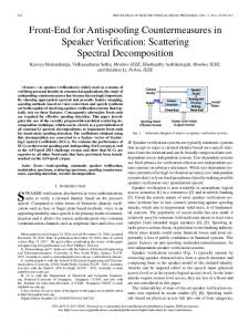
In the STFT the bandwidth of each filter is constant and related to the window function. The Q factor thus increases when moving from low to high frequencies since the absolute bandwidth f is identical for all filters. This is in contrast to the human perception system which is known to approximate a constant Q factor between 500Hz and 20kHz [21]. At least from a perceptual viewpoint, the STFT may thus not be universally ideal for the time-frequency analysis of speech signals. 3.3. The constant Q transform A more perceptually motivated time-frequency analysis known as the constant Q transform (CQT) was developed over the last few decades. The first was introduced in 1978 by Youngberg and Boll [22] with an alternative algorithm being proposed by Kashima and Mont-Reynaud Kashima [23]. In these approaches, octaves are geometrically distributed while the centre frequencies of each filter are linearly spaced. CQT was refined some years later in 1991 by Brown [24]. In contrast to the earlier work, the centre frequencies of each filter are also geometrically distributed, thereby following the equal-tempered scale [25] of western music. For this reason, Brown’s algorithm is widely used in music signal processing. The approach gives a higher frequency resolution for lower frequencies and a higher temporal resolution for higher frequencies. As illustrated in Figure 1, this is in contrast to the fixed time-frequency resolution of Fourier methods. From a perceptual point of view, geometrically spaced frequencies mean that
Δtk = Hk/fs t [s]
(b) CQT Figure 1: A comparison of the time-frequency resolution of the STFT (a) and CQT (b). For the STFT, the time and frequency resolutions, ∆t and ∆f , are constant. Here, H is the duration of the sliding analysis window (hop size). In contrast, the CQT employs a variable time resolution ∆tk (which is greater for higher frequencies) and a variable frequency resolution ∆fk (which is greater for lower frequencies). Now, the duration of the sliding analysis window Hk varies for each frequency bin. fs is the sampling rate and k is the frequency bin index. Red dots correspond to the filter bank centre frequencies fk (bin frequencies).
the centre frequency of every pair of adjacent filters has an identical frequency ratio and is perceived as being equally spaced. Over the last decade the CQT has been applied widely to the analysis, classification and separation of audio signals with impressive results, e.g. [26, 27, 28]. The CQT is similar to a wavelet transform with relatively high Q factors (∼100 bins per octave.) Wavelet techniques are, however, not well suited to this computation [29]. For example, methods based on iterative filter banks would require the filtering of the input signal many hundreds of times [30]. 3.4. CQT computation The CQT X CQ (k, n) of a discrete time domain signal x(n) is defined by: n+bNk /2c
X CQ (k, n) =
X
x(j)a∗k (j − n + Nk /2)
(3)
j=n−bNk /2c
where k = 1, 2, ..., K is the frequency bin index, a∗k (n) is the complex conjugate of ak (n) and Nk are variable window lengths. The notation b·c infers rounding down towards the
nearest integer. The basis functions ak (n) are complex-valued time-frequency atoms, defined according to: ak (n) =
1 n fk ( )exp[i(2πn + Φk )] C Nk fs
(4)
where fk is the center frequency of the bin k, fs is the sampling rate, and w(t) is a window function (e.g. Hann window). Φk is a phase offset. The scaling factor C is given by: bNk /2c
C=
X
� w
l=−bNk /2c
l + Nk /2 Nk
� (5)
Since a bin spacing corresponding to the equal-tempered scale is desired, the center frequencies fk obey: fk = f1 2
k−1 B
(6)
where f1 is the center frequency of the lowest-frequency bin and B determines the number of bins per octave. In practice, B determines the time-frequency resolution trade-off. The Q factor is then given by: Q=
fk = (21/B − 1)−1 fk+1 − fk
(7)
The window lengths Nk ∈ R in Equations 3 and 4 are realvalued and inversely proportional to fk in order that Q is constant for all frequency bins k, i.e.: Nk =
fs Q fk
(8)
The work in [31] introduced an additional parameter γ that gradually decreases the Q factors for low frequency bins in sympathy with the filters of the human auditory system. In particular, when γ = Γ = 228.7 ∗ (2(1/B) − 2(−1/B) ), the bandwidths equal a constant fraction of the ERB critical bandwidth [32]. Example CQT results are illustrated in Figure 2 which shows STFT and CQT-derived spectrograms for an arbitrarily selected speech signal from the ASVspoof database. The pitch F 0 of the utterance varies between 80Hz and 90Hz; the difference is only 10Hz. The frequency resolution of the conventional STFT is not sufficient to detect such small variations; 512 temporal samples at a sampling rate of 16kHz correspond to a spectral separation of 31.25Hz between two adjacent STFT bins. This same is observed for the second partial which varies between 160Hz and 180Hz where the difference is 20Hz. The spectral resolution of the STFT can of course be improved using a larger window, but to the detriment of time resolution. The CQT efficiently resolves these different spectral contents at low frequency.
4. CQCC extraction This section describes the extraction of constant Q cepstral coefficients. Cepstral analysis on CQT was already proposed by Brown [33] for the identification of musical instruments with a discrete success. Differently from Brown’s approach, our algorithm performs a linearisation of the frequency scale of the CQT, so that the orthogonality of the DCT basis is preserved. The discussion starts with a treatment of conventional cepstral analysis before the application to CQT.
Figure 2: Spectrograms of the utterance ‘the woman is a star who has grown to love the limelight’ for a male speaker in the ASVspoof database. Spectrograms computed with the shorttime Fourier Transform (top) and with the constant Q transform (bottom).
4.1. Conventional cepstral analysis The cepstrum of a time sequence x(n) is obtained from the inverse transformation of the logarithm of the spectrum. In the case of speech signals, the spectrum is usually obtained using the discrete Fourier transform (DFT) whereas the inverse transformation is normally implemented with the discrete cosine transform (DCT). The cepstrum is an orthogonal decomposition of the spectrum. It maps N Fourier coefficients onto q � N independent cepstrum coefficients that capture the most significant information contained within the spectrum. The Mel-cepstrum applies prior to cepstral analysis a frequency scale based on auditory critical bands [34]. It is the most common parametrisation used in speech and speaker recognition. Such features are referred to widely as Mel-frequency cepstral coefficients (MFCCs) which are typically extracted according to: "
M X
q m− M F CC(q) = log [M F (m)] cos M m=1
1 2
� # π
(9)
where the Mel-frequency spectrum is defined as M F (m) =
K 2 X DF T (k) Hm (k) X
(10)
k=1
where k is the DFT index, Hm (k) is the triangular weightingshaped function for the m-th Mel-scaled bandpass filter. M F CC(q) is applied to extract a number of coefficients less than the number of Mel-filters M . Typically, M = 25 and q varies between 13 and 20. 4.2. Constant Q cepstral coefficients Cepstral analysis cannot be applied using (6) directly since the k bins in X CQ (k) are on a different scale to those of the cosine function of the DCT; they are respectively geometrically
XCQ(k)
x(n) Constant-Q Transform
|XCQ (k)|2 Power spectrum
log|XCQ (k)|2
log|XCQ (l)|2
Uniform resampling
LOG
CQCC(p) DCT
Figure 3: Block diagram of CQCC feature extraction.
and linearly spaced. Inspired by the signal reconstruction works in [35, 36], this problem is solved here by converting geometric space to linear space. Since the k bins are geometrically spaced, the signal reconstruction can be viewed as a downsampling operation over the first k bins (low frequency) and as an upsampling operation for the remaining K − k bins (high frequency). We define the distance between fk and f1 = fmin as: � � k−1 ∆f k↔1 = fk − f1 = f1 2 B − 1 (11) where k = 1, 2, ..., K is the frequency bin index. The distance ∆f k↔1 increases as a function of k. We now seek a period Tl for linear resampling1 . This is equivalent to determining a value of kl ∈ 1, 2, ..., K such that: Tl = ∆f kl ↔1
(12)
To solve (12) we only need to focus on the first octave; once Tl is fixed for this octave, higher octaves will naturally have a resolution two times greater than that of the lower octave. A linear resolution is obtained by splitting the first octave into d equal parts with period Tl and by solving for kl : � � kl −1 1 f1 = f1 2 B − 1 → kl = Blog2 (1 + ) (13) d d The new frequency rate is then given by: � � ��−1 kl −1 1 Fl = = f1 2 B − 1 Tl
(14)
There are thus d uniform samples in the first octave, 2d in the second and 2j d in the (j − 1)th octave. The algorithm for signal reconstruction uses a polyphase antialiasing filter [37] and a spline interpolation method to resample the signal at the uniform sample rate Fl . Constant Q cepstral coefficients (CQCCs) can then be extracted in a more-or-less conventional manner according to: " � # L X p l − 12 π CQ 2 (15) CQCC(p) = log X (l) cos L l=1
where p = 0, 1, ..., L − 1 and where l are the newly resampled frequency bins. The extraction of CQCCs is summarised in Figure 3. Our Matlab implementation of CQCC extraction can be downloaded from http://audio.eurecom.fr/ content/software
5. Experimental setup The focus now returns to the assessment of spoofing countermeasures. Presented in the following is an overview of the experimental setup which includes the database, feature extraction and classifier configurations. 1 Whereas the period usually relates to the temporal domain, here it is in the frequency domain.
Table 2: The ASVspoof 2015 database: number of male and female speakers, number of genuine and spoofed speech utterances and data partitions.
Subset Training Development Evaluation
#Speakers Male Female 10 15 20
15 20 26
#Speakers Genuine Spoofed 3750 3497 9404
12625 49875 184000
5.1. ASVspoof 2015 database Table 2 summarizes the structure and contents of the ASVspoof 2015 database [16]. The database is structured into training, development and evaluation subsets. The three subsets contain both natural and spoofed speech for a number of different speakers. Spoofed material is derived from natural speech recordings by means of 10 different spoofing attacks (from S1 to S10). They take the form of popular speech synthesis and voice conversion algorithms (see [16] for details). In order to allow assessment of generalized countermeasures only attacks S1 to S5 are included in the training and development subsets. Attacks S6 to S10 are deemed as unknown attacks and contained only within the evaluation subset. All audio files are in PCM format with a 16kHz sampling rate and with a resolution of 16 bits per sample. 5.2. Feature Extraction The CQT is applied with a maximum frequency of Fmax = FN Y Q /2, where FN Y Q is the Nyquist frequency of 8kHz. The minimum frequency is set to Fmin = Fmax /29 ' 15Hz (9 being the number of octaves). The number of bins per octave B is set to 96. These parameters result in a time shift or hop of 8ms. Parameter γ is set to γ = Γ (see Section 4). Re-sampling is applied with a sampling period of d = 16. These parameters were all empirically optimised. Investigations using three different CQCC features dimensions are reported: 12, 19 and 29 all with appended C0 . The first two dimensions are chosen since they are common in speech and speaker recognition, respectively. The higher number is included to determine whether higher order coefficients contain any additional information useful for the detection of spoofing. From the static coefficients, dynamic coefficients, namely delta and delta-delta features are calculated and optionally appended to static coefficients, or used in isolation. Experiments were performed with all possible combinations of static and dynamic coefficients.
Table 3: System performance measured in terms of average EER (%) for the development set and for different feature dimensions and combinations of static and dynamic coefficients. S=static, D=dynamic, A=acceleration. Feature S D A SDA SD SA DA
12 + 0th
19 + 0th
29 + 0th
0.5233 0.4009 0.2085 0.2916 0.4271 0.4391 0.2079
0.3850 0.0942 0.0518 0.0947 0.2331 0.1564 0.0381
0.3619 0.0412 0.0100 0.0735 0.1622 0.0948 0.0154
5.3. Classifier Given the focus on features, all experiments reported in this paper use Gaussian mixture models (GMMs) in a standard 2class classifier in which the classes correspond to natural and spoofed speech. The two GMMs are trained on the genuine and spoofed speech utterances of the ASVspoof training dataset, respectively. We use 512-component models, trained with an expectation-maximisation (EM) algorithm with random initialisation. EM is performed until likelihoods converge. The score for a given test utterance is computed as the loglikelihood ratio Λ(X) = log L(X|θn ) − log L(X|θs ), where X is a sequence of test utterance feature vectors, L denotes the likelihood function, and θn and θs represent the GMMs for natural and spoofed speech, respectively. The use of GMM-based classifiers has been shown to yield among the best performance in the detection of natural and spoofed speech [12, 13].
6. Experimental results Presented in the following is an assessment of CQCC features for spoofing detection. This assessment is performed using the ASVspoof 2015 development subset. The attention then turns to an assessment of generalisation. Assessment is performed with the ASVspoof 2015 evaluation subset. 6.1. CQCC features Reported first is an evaluation of the proposed CQCC features using the ASVspoof development subset. Table 3 shows performance for different feature dimensions and 7 different combinations of static (S), delta (D) and acceleration (A) features. First, no matter that the combination, better performance is achieved with higher dimension features, indicating the presence of useful information in the higher order cepstra. Second, dynamic and acceleration coefficients give considerably better results than static coefficients. Acceleration coefficients give better results that dynamic coefficients, though for lower feature dimensions, their combination gives better performance than either alone. These observations are otherwise consistent across the different feature dimensions. The fact that dynamic and acceleration coefficients outperform static features seems reasonable given that spoofing techniques may not model well the more dynamic information in natural speech.
Table 4: System performance for known and unknown attacks measured in terms of average EER (%) for the evaluation set and for the 4 best system configurations found for the development set. #coef. Feat.
19 + 0th Known Unknown
A DA
0.0484 0.0228
0.4625 0.8263
29 + 0th Known Unknown 0.0185 0.0098
0.6724 0.8384
6.2. Generalisation The second goal of this work lies in the assessment of generalisation. This assessment is performed on the ASVspoof evaluation subset using feature dimensions of 19 and 29 with appended C0 and with A and DA combinations. Table 4 presents average EERs for known and unknown spoofing attacks in addition to the average. DA features consistently outperform A features for known spoofing attacks, while A outperform DA for unknown spoofing attacks for both feature dimensions. These results show that performance degrades significantly in the face of unknown attacks. This interpretation would be rather negative, however. Presented in the following is a comparison of CQCC to other results in the literature. These show that, even if performance for unknown spoofing attacks is worse than for known attacks, CQCC features still deliver excellent performance. 6.3. Comparative performance Table 5 shows the performance of CQCC independently for each of the different spoofing attacks grouped into known and unknown attacks. Results are presented here for only the 19th order feature set with A coefficients only. The average EER of this system is 0.26%. Also illustrated for comparison is the performance of the four systems described in Section 2.22 . Focusing first on known attacks, all four systems deliver excellent error rates of below 0.41%. The proposed CQCC features are third in the ranking according to the average error rate, with an EER of 0.05%. Voice conversion attacks S2 and S5 seem to be the most difficult to detect. Speech synthesis attacks S3 and S4, however, are perfectly detected by all systems. It is for unknown attacks where the difference between systems is greatest. Whereas attacks S6, S7 and S9 are detected reliably by all systems, there is considerable variation for attacks S8 and S10. In particular, the performance for attack S10, the only unit-selection-based speech synthesis algorithm, varies considerably; past results range from 8.2% to 26.1%. Being so much higher than the error rates for other attacks, the average performance for unknown attacks is dominated by the performance for S10. Average error rates for past work and unknown attacks range from 1.7% to 5.2%. CQCC features compare favourably. While the performance for S6, S7 and S9 is not as good as that of other systems, error rates are still low and below 0.1%. While the error rate for S8 of 1.0% is considerably higher than for other systems, it is significantly better than all other systems for attack S10. Here is the error is reduced to 1.1%. This corresponds to a relative 2 The authors thanks Md Sahidullah and Tomi Kinnunen from the University of Eastern Finland for kindly providing results independently for each spoofing attack.
Table 5: Performance in terms of average EER (%) for the best performing system, including individual results for each spoofing attack. Results for known and unknown attacks and the global average. Results for systems reviewed in Section 2 are included for comparison.
System CFCC-IF i-vector M&P feat. LFCC-DA CQCC-A
S1
S2
0.101 0.004 0.000 0.027 0.005
0.863 0.022 0.000 0.408 0.106
Known Attacks S3 S4 0.000 0.000 0.000 0.000 0.000
0.000 0.000 0.000 0.000 0.000
S5
Avg.
S6
S7
1.075 0.013 0.010 0.114 0.130
0.408 0.008 0.002 0.110 0.048
0.846 0.019 0.010 0.149 0.098
0.242 0.000 0.000 0.011 0.064
improvement of 87% with regard to the next best performing system for S10. The average performance of CQCC features for unknown attacks is 0.5%. This corresponds to a relative improvement of 72% over the next best system. The average performance across all 10 spoofing attacks is illustrated in the final column of Table 5. The average error rate of 0.26% is significantly better than those reported in previous work. The picture of generalisation is thus not straightforward. While performance for unknown attacks is worse than it is for known attacks, CQCC features nonetheless deliver the most consistent performance across the 10 different spoofing attacks in the ASVspoof database. Even if it must be acknowledge that the work reported in this paper was conducted postevaluation, to the authors’ best knowledge, CQCC features give the best spoofing detection performance reported to date.
7. Conclusions This paper introduces a new feature for the automatic detection of spoofing attacks which can threaten the reliability of automatic speaker verification. The new feature is based upon the constant Q transform and is combined with traditional cepstral analysis. Termed constant Q cepstral coefficients (CQCCs), the new features provide a variable-resolution, time-frequency representation of the spectrum which captures detailed characteristics which are missed by more classical approaches to feature extraction. These characteristics are shown to be informative for spoofing detection. When coupled with a simple Gaussian mixture model-based classifier and assessed on a standard database, CQCC features outperform all existing approaches to spoofing detection. In addition, while there is still a marked discrepancy between performance for known and unknown spoofing attacks, CQCC results correspond to a relative improvement of 72% over the previously best performing system. Future work should consider the application of CQCCs for more generalised countermeasures such as a 1-class classifier. The application of CQCCs in other speaker recognition and related problems is another obvious direction.
8. Acknowledgements The paper reflects some results from the OCTAVE Project (#647850), funded by the Research European Agency (REA) of the European Commission, in its framework programme Horizon 2020. The views expressed in this paper are those of the authors and do not engage any official position of the European Commission.
Unknown Attacks S8 S9 0.142 0.015 0.000 0.074 1.033
0.346 0.004 0.000 0.027 0.053
S10
Avg.
All Avg.
8.490 19.57 26.10 8.185 1.065
2.013 3.922 5.222 1.670 0.462
1.211 1.965 2.612 0.890 0.255
9. References [1] N. Evans, T. Kinnunen, and J. Yamagishi, “Spoofing and countermeasures for automatic speaker verification,” in INTERSPEECH, 2013, pp. 925–929. [2] Z. Wu, N. Evans, T. Kinnunen, J. Yamagishi, F. Alegre, and H. Li, “Spoofing and countermeasures for speaker verification: A survey,” Speech Communication, vol. 66, pp. 130 – 153, 2015. [3] J. Lindberg and M. Blomberg, “Vulnerability in speaker verification – a study of technical impostor techniques,” in Proc. European Conference on Speech Communication and Technology (Eurospeech), 1999. [4] J. Villalba and E. Lleida, Biometrics and ID Management: COST 2101 European Workshop, BioID 2011, Brandenburg (Havel), Germany, March 8-10, 2011. Proceedings, chapter Detecting Replay Attacks from Far-Field Recordings on Speaker Verification Systems, pp. 274–285, 2011. [5] B. L. Pellom and J. H. L. Hansen, “An experimental study of speaker verification sensitivity to computer voice-altered imposters,” in Proc. IEEE International Conference on Acoustics, Speech, and Signal Processing (ICASSP), Mar 1999, vol. 2, pp. 837–840 vol.2. [6] P. Z. Patrick, G. Aversano, R. Blouet, M. Charbit, and G. Chollet, “Voice forgery using ALISP: Indexation in a client memory,” in Proc. IEEE International Conference on Acoustics, Speech, and Signal Processing (ICASSP), March 2005, vol. 1, pp. 17–20. [7] Takashi Masuko, Takafumi Hitotsumatsu, Keiichi Tokuda, and Takao Kobayashi, “On the security of HMM-based speaker verification systems against imposture using synthetic speech,” in In Proceedings of the European Conference on Speech Communication and Technology, 1999, pp. 1223–1226. [8] P. L. De Leon, M. Pucher, J. Yamagishi, I. Hernaez, and I. Saratxaga, “Evaluation of speaker verification security and detection of HMM-based synthetic speech,” Audio, Speech, and Language Processing, IEEE Transactions on, vol. 20, no. 8, pp. 2280–2290, Oct. 2012. [9] Y. W. Lau, M. Wagner, and D. Tran, “Vulnerability of speaker verification to voice mimicking,” in Proceedings of 2004 International Symposium on Intelligent Multimedia, Video and Speech Processing, 2004., Oct 2004, pp. 145–148. [10] Y. W. Lau, D. Tran, and M. Wagner, Knowledge-Based Intelligent Information and Engineering Systems: 9th International Conference, KES 2005, Melbourne, Australia, September 14-16, 2005, Proceedings, Part IV, chapter
Testing Voice Mimicry with the YOHO Speaker Verification Corpus, pp. 15–21, Springer Berlin Heidelberg, Berlin, Heidelberg, 2005. [11] Z. Wu, T. Kinnunen, N. Evans, J. Yamagishi, C. Hanilci, M. Sahidullah, and A. Sizov, “ASVspoof 2015: the first automatic speaker verification spoofing and countermeasures challenge,” in INTERSPEECH, Dresden, Germany, 2015. [12] T. B. Patel and H. A. Patil, “Combining evidences from mel cepstral, cochlear filter cepstral and instantaneous frequency features for detection of natural vs. spoofed speech,” in INTERSPEECH, 2015, pp. 2062–2066. [13] Md. Sahidullah, T. Kinnunen, and C. Hanilc¸i, “A comparison of features for synthetic speech detection,” in INTERSPEECH, 2015, pp. 2087–2091. [14] C. Hanilc¸i, T. Kinnunen, Md. Sahidullah, and A. Sizov, “Classifiers for synthetic speech detection: a comparison,” in INTERSPEECH, 2015, pp. 2087–2091. [15] F. Alegre, R. Vipperla, A. Amehraye, and N. Evans, “A new speaker verification spoofing countermeasure based on local binary patterns,” in INTERSPEECH, Lyon, FRANCE, 08 2013.
[25] R. E. Radocy and J. D. Boyle, Psychological foundations of musical behavior, C. C. Thomas, 1979. [26] G. Costantini, R. Perfetti, and M. Todisco, “Event based transcription system for polyphonic piano music,” Signal Process., vol. 89, no. 9, pp. 1798–1811, Sept. 2009. [27] R. Jaiswal, D. Fitzgerald, E. Coyle, and S. Rickard, “Towards shifted nmf for improved monaural separation,” in 24th IET Irish Signals and Systems Conference (ISSC 2013), June 2013, pp. 1–7. [28] C. Schorkhuber, A. Klapuri, and A. Sontacch, “Audio pitch shifting using the constant-Q transform,” Journal of the Audio Engineering Society, vol. 61, no. 7/8, pp. 425– 434, July/August 2013. [29] S. Mallat, A Wavelet Tour of Signal Processing, Third Edition: The Sparse Way, Academic Press, 3rd edition, 2008. [30] M. Vetterli and C. Herley, “Wavelets and filter banks: theory and design,” IEEE Transactions on Signal Processing, vol. 40, no. 9, pp. 2207–2232, Sep 1992.
[16] Z. Wu, T. Kinnunen, N. Evans, and J. Yamagishi, “ASVspoof 2015: the first automatic verification spoofing and countermeasures challenge evaluation plan,” 2014.
[31] C. Sch¨orkhuber, A. Klapuri, N. Holighaus, and M. D¨orfler, “A Matlab toolbox for efficient perfect reconstruction time-frequency transforms with log-frequency resolution,” in Audio Engineering Society (53rd Conference on Semantic Audio), G. Fazekas, Ed., AES (Vereinigte Staaten (USA)), 6 2014.
[17] S. Novoselov, A. Kozlov, G. Lavrentyeva, K. Simonchik, and V. Shchemelinin, “STC anti-spoofing systems for the asvspoof 2015 challenge,” in INTERSPEECH, 2015.
[32] B. R. Glasberg and B. C. J. Moore, “Derivation of auditory filter shapes from notched-noise data,” Hearing Research, vol. 47, no. 1, pp. 103 – 138, 1990.
[18] X. Xiao, X. Tian, S. Du, H. Xu, E. Chng, and H. Li, “Spoofing speech detection using high dimensional magnitude and phase features: the NTU approach for ASVspoof 2015 challenge,” in INTERSPEECH, 2015. [19] D. Gabor, “Theory of communication,” J. Inst. Elect. Eng., vol. 93, pp. 429–457, 1946.
[33] J. Brown, “Computer identification of musical instruments using pattern recognition with cepstral coefficients as features,” The Journal of the Acoustical Society of America, vol. 105, no. 3, pp. 1933–1941, 1999.
[20] A. V. Oppenheim, R. W. Schafer, and J. R. Buck, Discretetime Signal Processing (2Nd Ed.), Prentice-Hall, Inc., Upper Saddle River, NJ, USA, 1999.
[34] S. Davis and P. Mermelstein, “Comparison of parametric representations for monosyllabic word recognition in continuously spoken sentences,” IEEE Transactions on Acoustics, Speech and Signal Processing, vol. 28, no. 4, pp. 357–366, Aug 1980.
[21] B. C. J. Moore, An Introduction to the Psychology of Hearing, BRILL, 2003.
[35] G. Wolberg, Cubic Spline Interpolation: a Review, Columbia University, 1988.
[22] J. Youngberg and S. Boll, “Constant-q signal analysis and synthesis,” in IEEE International Conference on Acoustics, Speech, and Signal Processing (ICASSP), Apr 1978, vol. 3, pp. 375–378.
[36] S. Maymon and A. V. Oppenheim, “Sinc interpolation of nonuniform samples,” IEEE Transactions on Signal Processing, vol. 59, no. 10, pp. 4745–4758, Oct 2011.
[23] B. Mont-Reynaud, “The bounded-Q approach to timevarying spectral analysis,” 1986. [24] J. Brown, “Calculation of a constant Q spectral transform,” Journal of the Acoustical Society of America, vol. 89, no. 1, pp. 425–434, January 1991.
[37] P. Jacob, “Design and implementation of polyphase decimation filter,” International Journal of Computer Networks and Wireless Communications (IJCNWC), ISSN, pp. 2250–3501.