selection for faulty neural networks have been published. Thus, the paper derive a ..... autoregressive (NAR) time series prediction problems. In the simulations ...
International Journal of Intelligent Systems and Technologies 4:1 2009
Regularization Parameter Selection for Faulty Neural Networks Hong-jiang Wang, Fei Ji, Gang Wei, Chi-Sing Leung, and Pui-Fai Sum
Traditional methods of choosing the regularization parameter is the test set method or cross-validation [5]-[7], i.e., calculating the prediction error with the testing or training dataset for each the candidate regularization parameter and then selecting the optimal regularization parameter with the minimum prediction error value. However, when the network suffers from the multi-node open fault, i.e., multiple nodes synchronously take no effect in the training process [8], the above operation process has to be repeated for each faulty network pattern and then the mean prediction error (MPE) is calculated, which will cost a lot of dealing time. In addition, though some statistical methods have been proposed to evaluate the mean prediction error, e.g., Moody’s GPE [9], most of them aim at the fault-free neural networks. To our best knowledge, no literatures about regularization parameter selection for faulty neural networks have been published. Thus, the paper derive a formula, called as MPE formula, to evaluate the mean prediction error for faulty neural networks in multi-node open fault conditions based on Moody’s thinking and then use it to choose the optimal regularization parameter. Simulation results show that our proposed MPE formula can quickly find the optimal regularization parameter, which is very close to the actual one by the test set method.
Abstract—Regularization techniques have attracted many researches in the past decades. Most focus on designing the regularization term, and few on the optimal regularization parameter selection, especially for faulty neural networks. As is known that in the real world, the node faults often inevitably take place, which would lead to many faulty network patterns. If employing the conventional method, i.e., the test set method or cross-validation, to find the optimal regularization parameter, it will cost a lot of time. Moreover, although some statistic methods have been proposed, almost of them aim at the fault-free networks. Thus, in the paper, a MPE formula is derived to evaluate the mean prediction error in the multi-node open fault situations and then used to select the optimal regularization parameter. Experiment results have shown that the optimal parameter value selected by our proposed formula is very close to the actual one, chosen by the conventional test set method. Our contribution is that our proposed MPE formula can be used in choosing the regularization parameter instead of the test set method for faulty neural networks with multi-node open fault.
Keywords—Faulty neural networks, multi-node open fault, regularization parameter, mean prediction error. I. INTRODUCTION
A
S is
known that the node faults inevitably take place in the real application for neural networks, especially in VLSI [1]. Without the special care, the fault situation could result in drastic performance degradation [2]. Due to the simplicity of computation and structure, regularization methods have been considered as one of the most effective techniques for improving the fault tolerant through adding one regularization term, consisting of regularization parameter and regularization matrix, in the objective function [3]. The regularization parameter plays an important role in the regularization method and controls the overfitting or underfitting of the network learning process. If the improper regularization parameter is selected, the network learning performance, i.e., generalization, will suffer from the drastic degradation [4]. Thus, it is necessary to choose a proper regularization parameter for improving the generalization performance of faulty neural network with the regularization method.
II. FAULTY NEURAL NETWORKS In the section, we shall present the basic framework of the faulty neural networks. A. RBF model We consider the RBF network model as an example. For clarity, the bold letter denotes the vector in the paper. Thus, the unknown function mapping f (⋅) can be approximated as [10] ∧
M
f ( x ) ≈ f ( x, w ) = ∑ w jφ j ( x ) = ΦT ( x ) w ,
(1)
j =1
where x = [ x1 ,x2 ," ,xN ] is the training input dataset, those corresponding output dataset y = [ y1 , y2 ," , y N ] can be written by y = f (x) + n , n is the independent identity distribution Gaussian random noise vector with mean zero and variance
σ n2
Hongjiang Wang, Fei Ji, and Gang Wei are with the School of Electronic and Information Engineering, South China University of Technology, Guangzhou, China (Phone: 086-020-87113038; e-mail: eehjwang@ hotmail.com). Chi-Sing Leung is with the Electrical Engineering Department, City University of HongKong, HongKong. Pui-Fai Sum is with National Chung Hsing University, Taiwan.
. w = [ w1 , w2 ," , wM ] is the RBF weight vector,
and φ j ( x ) = exp
( x−c
2 j
)
/ Δ is the j th kernel function of
RBF, Φ(x) = [φ1 (x), φ2 (x)," , φM (x)] , 45
⋅ is the matrix norm,
International Journal of Intelligent Systems and Technologies 4:1 2009
c j ’s are the center of RBF, Δ is the kernel width of RBF.
mean testing error for faulty networks E test ( w, b ) is
B. Faulty model The existing literatures often discuss two kinds of fault models, i.e., multi-node open fault [8] and multiplicative weight noise [11], [12]. In the paper, we mainly consider the multi-node open fault situation, where the node fault means that the corresponding weights are equal to zero. Therefore, the faulty weight vector is l = b⊗w, (2) w where ⊗ is the element-wise multiplication operator,
, (6) N where M is the effective number of weights in the RBF eff
model, S e is the measured noise variance, the first term is the mean training error for faulty networks. Moreover, according to the definition of M eff in [9], we get
N 2
M eff =
b = [b1 , b2 ," , bM ] is the node fault vector with bi ∈ [0,1] . Moreover, when bi = 0 , the i th node is out of work. T
M
i =1
=1
−1
i
=1
,
i
(7)
∂ 2 Etrain 2 = − φα ( xi ) , ∂yi ∂wα N
Tβ i =
∂ 2 Etrain 2 = − φβ ( xi ) , N ∂wβ ∂yi
Uαβ =
∂ 2 E ( w, b ) = 2 ( Hφ + pR ) . ∂wα ∂wβ
(
M eff = trace Hφ ( Hφ + pR )
−1
).
(8)
In addition, the mean train error for faulty neural networks can be expressed as
E train ( w , b ) = = =
∑( y −Φ
1 N
∑ ( y − Φ ( x )( b ⊗ w ) )
1 N
N
T
i
i =1
i) ( xi ) w
2
1 N
N
2
(9)
T
i
i =1
N
∑y i =1
2 i
i
− 2 (1 − p ) ⋅
1 N
∑( y ⋅Φ (x )w) N
T
i
i =1
i
+ (1 − p ) w T ( Hφ + pR ) w
III. MEAN PREDICTION ERROR
and the mean training error for fault-free neural networks is
The regularizer for faulty RBF neural networks with multi-node open fault proposed by Leung et al. is λ w T Rw , where R = G − H φ is the regularization matrix, λ is the 1 N Hφ = ∑ φ ( x j ) φ T ( x j ) N j =1
Etrain ( w ) =
1 N
∑ ( yi − ΦT ( xi ) w ) N
2
(10)
i =1
1 N 2 1 N yi − 2 ⋅ ∑ ( yi ⋅ ΦT ( xi ) w ) + w T Hφ w ∑ N i =1 N i =1 Thus, comparing (9) and (10), we can get 1 N E train ( w, b ) = (1 − p ) Etrain ( w ) + p ⋅ ∑ yi2 N i =1 . (11) =
and
G = diag ( Hφ ) . Therefore, the error objective function for
faulty neural networks with multi-node open fault can be expressed as 2 1 N (4) E ( w, λ ) = ∑ yi − ΦT ( xi ) w + λ w T Rw , N i =1 and the training error Etrain ( w ) is
(
M
Tiα =
Therefore,
C. Regularization learning Generally speaking, the regularization method employs a regularization term to limit weight magnitude since the large weights have a big effect on the output of the neural network. As one of the most common regularizers, the weight decay has been widely researched and applied in the past years. Studies have shown that weight decay regularizer to some extend can improve the fault tolerant in the faulty neural networks, but it is not the best one [8]. Hence, Leung et al. have developed a new regularizer, which has a better ability to tolerate the multi-node open fault than others, e.g., the standard weight decay [16].
parameter,
N
T αU αβ Tβ ∑∑∑ α β
where
Otherwise, the i th one works. p is the node fault rate with the following relation ⎧⎪ 1 − p, if i = i ' . (3) bi bi ' = ⎨ 2 ' i 1 p , if i − ≠ ( ) ⎪⎩ To enhance the fault tolerant of the faulty neural networks, some methods have been proposed, such as injecting weight noise during training [13], adding the node redundancy [14] and regularization [15] and so on.
regularization
M eff
E test ( w, b ) = E train ( w, b ) + 2Se
+ ( p − p 2 ) wT Rw
)
Thereby, substituting (8) and (11) into (6), we have
MPE = E test ( w, b ) = (1 − p ) Etrain ( w )
2
+p⋅
1 N (5) Etrain ( w ) = ∑ ( yi − ΦT ( xi ) w ) . N i =1 Following the Moody’s thinking [9], we can know that the
1 N
∑ y +( p − p )w N
i =1
2 i
(
2
T
Rw
−1 2S + e trace Hφ ( Hφ + pR ) N
46
)
(12)
International Journal of Intelligent Systems and Technologies 4:1 2009
the test set method.
Using the MPE formula, we can rapidly obtain the MPE value and select the optimal regularization parameter.
0.018
IV. SIMULATIONS
parameter as λ = ⎡⎣10 ,10 −4
−3.95
testing error
To test our theoretic results, two function approximation examples have been employed, i.e., sinc function and nonlinear autoregressive (NAR) time series prediction problems. In the simulations, firstly, we use our proposed formula method, MPE formula, and the test set method to calculate the testing error values of each the candidate regularization parameter λ , and then take the optimal parameter value with the minimal testing error value, respectively. Finally, two results have been compared to verify our theoretic results. Therefore, to get the best test results, it is important to select the approximate candidate regularization parameter. Taking the tradeoff of the complexity and accuracy, we set the candidate regularization
MPE test set 0.012
-3
10
-2
-1
10
10
λ
(a) p = 0.05 0.018
, " ,10 ⎤⎦ . Moreover, we random 0
y − Φ T (x)w N −M
testing error
generate 10000 faulty networks to calculate the actual MPE with the test set method. In addition, the variance of measured noise Se can be obtained using the Fedorov’s method [17], i.e., Se =
0.015
0.015
2
.
(10) MPE test set 0.012
A. One-dimension function approximation The sinc function approximation problem is a benchmark one-dimension function learning example [18]. The function relation equation can be generated by (11) y = sinc(x) + n . where n is the independent identity distribution Gaussian random noise vector with mean zero and variance 0.01. In simulation, 200 training dataset and 1000 testing dataset are generated. The RBF network model has 37 nodes, which are taken uniformly between -4.5 and 4.5. In addition, the kernel width value of RBF network is 0.49 according to Sum’s method in [19]. Our task is to find and compare the optimal regularization parameters for two methods, i.e., MPE formula and the test set method. Fig.1 has shown simulation results for the sinc function approximation example using two evaluation methods, i.e., MPE formula and test set method. From the figures, we can see that the optimal regularization parameters selected by the two methods are very close. For example, when the fault rate is equal to 0.05, the chosen regularization parameter for two methods are both about 0.056234. Moreover, we have repeated the simulations for 50 times and found the range of optimal regularization parameter values chosen by the MPE formula is around from 0.050119 to 0.063096. In addition, to deeply affirm our results, we set the fault rate as 0.1 and repeat the above training and testing process. The similar curve shapes can be observed in fig.1(b), i.e., the lowest points of two curves almost are in one vertical line as well. Therefore, we can find that no matter how the fault rate varies, the optimal regularization parameter selected by our proposed formula is very close to the one by the conventional method, i.e.,
-3
10
-2
-1
10
10
λ
(b) p = 0.1 Fig. 1 Optimal regularization parameter selection for sinc function approximation example with the different methods, i.e., MPE formula and test set method.
B. Multi-dimension function approximation We consider the nonlinear autoregressive time series example as the multi-dimension function approximation problem [20]. Those function expression can be given as
( − ( 0.3 + 0.9 exp ( − y
) ( i − 1) ) ) y ( i − 2 ) ,
y ( i ) = 0.8 − 0.5exp ( − y 2 ( i − 1) ) y ( i − 1) 2
(12)
+0.1sin (π y ( i − 1) ) + n ( i ) where n ( i ) is a mean-zero Gaussian random variable with variance 0.01. The RBF model is to predict y ( i ) based on y ( i − 1) and y ( i − 2 ) , i.e., x ( i ) = ⎣⎡ y ( i − 1) , y ( i − 2 ) ⎦⎤ . In
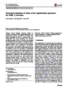
simulation, 500 training dataset and 500 testing dataset are generated based on the initial setting, y ( 0 ) = y ( −1) = 0 . Moreover, the Chen’s LROLS method is applied to select important RBF centers [21]. The number of selected nodes is 40. Fig.2 has shown the simulation results for the NAR time series prediction with two evaluation methods, i.e., MPE formula and the test set method, when p = 0.05 or p = 0.1 . From the figures, we can find that the regularization parameters 47
International Journal of Intelligent Systems and Technologies 4:1 2009 [2]
chosen by the MPE formula are very close to that by the test set method. For instance, in fig.2(a), when the fault rate is equal to 0.05, the selected regularization parameter for two methods are both about 0.063096. Furthermore, we have repeated the simulations for 50 times and found the range of optimal regularization parameter values chosen by the MPE formula is around from 0.056234 to 0.070795. In addition, we can obtain the similar results from fig.2(b).
[3]
[4] [5]
[6]
0.6
testing error
[7]
[8]
0.56
[9] MPE test set 0.52
-3
10
-2
10
[10]
-1
10
λ
[11]
(a) p = 0.05 0.7
[12]
testing error
[13] [14] 0.6
[15]
[16]
MPE test set 0.5
-3
10
-2
10
[17] [18]
-1
10
λ
(b) p = 0.1 Fig. 2 Optimal regularization parameter selection for nonlinear autoregressive time series prediction example with the different methods, i.e., MPE formula and test set method.
[19]
V. CONCLUSION
[21]
[20]
The paper derives a MPE formula to find the optimal regularization parameter for faulty neural networks. Simulation results have shown that our proposed formula method can quickly find the optimal regularization parameter, which is very close to the actual one by the conventional method, i.e., the test set method. It implies that ones can selection the optimal regularization parameter using our MPE formula instead of the test set method for faulty neural networks.
Hong-Jiang Wang: received the B.Eng. in Electrical and Electronic Engineering from Ningbo University in 2000, M.Phil. and Ph.D. in Electronic and Information Engineering from South China University of Technology in 2004 and 2007. He is currently a research assistant in the Department of Electronic Engineering, City University of Hong Kong. In addition, in between 2000 to 2002, he had worked as an arithmetic researcher in the institute of mobile communication technology research of Ningbo University. His current research interests include neural computation, Ad Hoc networks and wireless ultra-wideband communication.
ACKNOWLEDGMENT The work is supported by the grant from National Science Fund for Distinguished Young Scholars (No. 60625101). REFERENCES [1]
G.R. Bolt. Fault Tolerance in Artificial Neural Networks. PhD thesis, University of York, 1992. K. Hagiwara, K. Kuno. Regularization learning and early stopping in linear networks. International Joint Conference on Neural Networks, Como, Italy, 4:511-516, 2000. C.M. Bishop. Neural Networks for Pattern Recognition. Oxford, UK: Oxford University Press, 1995. J. Moody. Prediction Risk and Neural Network Architecture Selection. From Statistics to Neural Networks: Theory and Pattern Recognition Applications, NATO ASI Series F, Springer-Verlag, 1994. S.I. Amari, N. Murata, K.R. Muller, M. Finke, and H.H. Yang. Asymptotic statistical theory of overtraining and cross-validation. IEEE Trans. Neural Networks, 8:996-985, 1997. Ping Guo, Michael R. Lyu, and C. L. Philip Chen. Regularization Parameter Estimation for Feedforward Neural Networks. IEEE Tran. Systems, Man, and Cybernetics—PART B: Cybernetics, 33(1):35-44, 2003. Z. Zhou, S. Chen, Z. Chen. Improving tolerance of neural networks against multi-node open fault. International Joint Conference on Neural Networks. 3:1687-1692, 2001. J.E. Moody. Note on generalization, regularization and architecture selectionin nonlinear learning systems. Neural Networks for Signal Processing, 1-10, 1991. M. J. L. Orr. Introduction to Radial Basis Function Networks. Http://www.anc.ed.ac.uk/ mjo/papers/intro.ps, 1996. M.A. Jabri and B. Flower. Weight perturbation: An optimal architecture for analog VLSI feedforward and recurrent multi-layer networks. IEEE Trans. Neural Networks, 3(1):154-157, 1992. Ping Man Lam, Chi-Sing Leung, and Tien Tsin Wong. Noise-resistant fitting for spherical harmonics. IEEE Trans. Visualization and Computer Graphics, 12(2):254-265, 2006. K. Matsuoka. Noise injection into inputs in back-propagation learning. IEEE Trans. Systems, Man and Cybernetics, 22(3):436-440, 1992. M.D. Emmerson. Fault Tolerance and Redundancy in Neural Networks. PhD thesis, University of Southampton, 1992. Chi-Sing Leung, A.C. Tsoi, and L.W. Chan. On the regularization of forgetting recursive least square. IEEE Trans. Neural Networks, 12:1314-1332, 2001. Chi-Sing Leung, John Sum. A Fault-Tolerant Regularizer for RBF Networks. IEEE Transactions Neural Networks, 19(3): 493-507, 2008. V.V. Fedorov. Theory of optimal experiments. Academic Press, 1972. S. Chen, X. Hong, C.J. Harris, and P.M. Sharkey. Sparse modeling using orthogonal forward regression with press statistic and regularization. IEEE Trans. Systems, Man and Cybernetics, Part B, 898-911, 2004. J.-F. Sum, C.-S. Leung, K.-J. Ho. On objective function, regularizer, and prediction error of a learning algorithm for dealing with multiplicative weight noise. IEEE Trans. Neural Networks, 20(1):124-138, 2009. M. Mackey, L. Glass. Oscillation and chaos in physiological control systems. Science, 197(4300):287-289, 1977. Chen, S., 2006. Local regularization assisted orthogonal least squares regression. Neurocomputing 69 (4-6), 559–585.
A. Hamilton, S. Churcher, P.J. Edwards, et al.. Pulse stream VLSI circuits and systems: The EPSILON neural network chipset. International Journal of Neural Systems, 4(4):395-405, 1993.
48