Conformal Method for Quantitative Shape Extraction: Performance Evaluation George Kamberov Stevens Institute of Technology Department of Computer Science Hoboken, NJ 07030
[email protected]
Abstract We evaluate our recently developed conformal method for quantitative shape extraction from unorganized 3D oriented point clouds. The conformal method has been tested previously on real, noisy, 3D data. Here we focus on the empirical evaluation of its performance on synthetic, ground truth data, and comparisons with other methods for quantitative extraction of mean and Gauss curvatures presented in the literature.
1. Introduction The reliable extraction of quantitative geometric descriptors from a discrete cloud of points sampled from a surface is a fundamental task in computer graphics and computer vision. One approach is to begin by fitting, possibly locally, a smooth, parameterized or implicit surface, or a polygonal mesh to the point cloud; the next step is to apply the standard differential geometric formulae on the smooth surface, or one of the numerous methods for estimating shape descriptors on a polygonal surface. (See for example [7, 3, 6, 10, 12, 13, 15, 14].) These methods involve non-stable computations – second order numeric differentiation over unreliable and sparse data and numeric diagonalization of general matrices with noisy entries. The ”differentiation free” curvature estimates underlying some of the methods, for example, the normal curvature estimate popularized in [15] degrade on sparse or very curved data sets. The results on real, noisy and/or sparse data are unsatisfactory [13, 16, 6, 8]. A popular way to improve the stability of the estimates is to smooth the data but this leads to distortion of features and to systematic errors in curvature estimates [16]. A recent study [14] indicates that even on synthetic data the performance of some of the most popular algorithms is uneven and hardly accurate. The estimation of shape descriptors from point clouds involves three sub-tasks: cloud orientation – estimating the
Gerda Kamberova Hofstra University Department of Computer Science Hempstead, NY 11549
[email protected]
normals at each 3D sample point; topologizing the point cloud, that is, estimating the ”nearest neighbors” of each 3D sample point; computing shape descriptors at each point. Estimating the orientation and topology/connectivity of a point cloud is the subject of intensive research, [2, 7, 1, 9, 11, 17, 12, 19]. The conformal method (CM), we introduced in [18], estimates quantitatively mean and Gauss curvatures, and principal curvature directions on an topologized, oriented cloud (that is a cloud of points with a neighborhood and a normal attached at each point). CM does not use models, parameterizations, or triangulations, and nonstable numeric operations. No smoothing of the data is required. Numeric errors and noise are addressed by redundant estimates of the geometric descriptors at each point. All the computations are local – so the method can be efficiently implemented as a parallel algorithm with low synchronization overhead. In this paper we outline the CM, then we evaluate its performance on synthetic ground truth data, and compare it against the methods investigated in [6, 14] and the results obtained by using the classical differential geometric formulae which involve explicit diagonalization of the second fundamental form [5]. We refer to the last approach as the standard method (SM). The SM is the basis for many of the popular algorithms.
2. The Conformal Method We introduced the conformal method (CM) in [18]. The limited space does not allow us to present details. We simply summarize the main definitions and observations here. The conformal method is based on a discrete versions of basic identities in the conformal geometry of a parameterized oriented surface S = f (M ), f : M → R3 , where M is an oriented two-dimensional domain. We denote by df the differential of f , by N : M → R3 its Gauss map, and by J, the associated complex structure defined so that for every vector v tangent to M , J(v) is the vector tangent to M such that df (J(v)) = N × df (v). The second fundamen-
tal form of f is defined by II(u, v) = − < dN(u)|df (v) > where < ·|· > is the Euclidean scalar product in R3 . At every point p ∈ M there exists a positively oriented orthonormal frame {e1 , e2 = J(e1 )} , kdf (ei )k = 1, of the tangent plane at p, such that the symmetric quadratic form II(·, ·) is represented by a diagonal matrix diag (κ1 , κ2 ). The vectors e1 and e2 are called principal curvature vectors, they define the principal axes. The numbers κ1 , κ2 are the principal curvatures, their average is the mean curvature, H, and their product is the Gauss curvature K. The mean curvature, H, satisfies 1 H = − hdf (u)|dN(u) − N × dN(J(u))i 2
at P . For every adapted frame φ = (u, v) let, w = 0.5 (dN(u) + N × dN(v)), Auu =< w|u >, Auv =< w|v >, and µ ¶ Auu Auv Aφ = Auv −Auu Last, A is the average of Aφ (but represented in the common basis v1 , v2 ), and e1 , e2 are the eigenvectors of A. The Gauss Curvature K: The definition follows the same pattern as the definitions of the mean curvature and the principal axes. It is based on discrete differences versions of basic identities for smooth surfaces but it uses the estimated mean curvature and (4). For every adapted frame φ let w = 0.5 (dN(u) + N × dN(v)), Auu =< w|u >, Auv =< w|v >, and λ2φ = A2uu + A2uv . Last, λ2 is the average of all λ2φ , and the Gauss curvature K = H 2 − λ2 .
(1)
for every tangent vector u such that |df (u)| = 1. Thus H can be immediately computed if one knows the 3D vectors df (u), dN(u), and dN(J(u)). The 1-form ω defined by ω
=
1 (dN + N × dN ◦ J) . 2
(2)
3. Results and Comparisons
holds the key to computing the Gauss curvature and the principal curvature directions. Indeed, let µ ¶ a b A= (3) b −a
We have tested the performance of the conformal method (CM) on real, 3D point clouds obtained via laser range scanners, CT 3D medical data, and stereo reconstruction, [18]. Here we test the performance of the CM on synthetic data with ground truth mean and Gauss curvature values. Note the input data are not subject to any preprocessing or smoothing. In the following subsections we investigate the performance of the conformal method against various methods for quantitative extraction of mean and Gauss curvatures presented in the literature.
be the two by two matrix defined by representing the quadratic form < ω(·)|df (·) > with respect to an arbitrary positively oriented basis (u, v) of tangent vectors to M . The Gauss curvature, K, satisfies K = H 2 − (a2 + b2 ).
(4)
3.1. Methods Presented in [14]
The principal curvature directions are expressed explicitly in terms of the coefficients ©a and b. For the rest ª of this paper we assume that M = (p, N) ∈ R3 × S 2 is an oriented point cloud equipped with topology. For every point P = (p, N) ∈ M we denote the by Tp M , the plane perpendicular to N at p, and by U(P ) the neighborhood of P in the cloud. With every Qi ∈ U = U(P ) we associate a positively oriented adapted frame φi = (ui , vi ) of the plane Tp M. Here ui is the unit vector in direction of the −→i = qi − p on Tp M orthogonal projection of the vector pq and vi = N × ui . Mean Curvature H, at P : First, for every adapted frame φ = (u, v), the vector w = 0.5 (dN(u) − N × dN(v)) is computed, next Hφ = − < w|u >, last, some form of statistical averaging is used over the neighborhood to estimate the mean curvature of the surface at the oriented point P as the average of the sample measurements, Hφ , defined for each adapted frame φ at the point. The sample variance is kept as a measure of the reliability in the estimate. Principal Curvature Axes e1 and e2 , at P : Let v1 , v2 be an orthonormal basis in the tangent plane
The CM is evaluated on synthetic ground truth data provided at a site at Technion Institute, Israel; see [14]. Six different types of triangulated surfaces are considered, a sphere, a cylinder, a cone, an ellipsoid, a surface of revolution, the Utah teapot body, and the Utah teapot spout. Ground truth data are provided at the vertices: those are mean curvature squared and Gauss curvature. The surfaces are sampled at five to seven different levels of resolution, the triangulation is given (each level of resolution has increasing number of triangles used for the polyhedral approximation of the surface). We have used the neighborhood information from the global triangulation provided. The normal at each vertex is approximated by averaging the normals to the triangles adjacent to the vertex. Figure 1 shows examples of cloud points for the surface of revolution and the Utah teapot – the surfaces for which results were presented in [14]. In [14] nine methods for quantitative shape extraction of mean and Gauss curvatures are compared. The methods are based on Taubin’s approach, the angular deficit approach, 2
0.16
2.5 0.14
0.12
2
0.1
1.5 0.08
0.06
1
Figure 1. Sample oriented point clouds for the surface of 0.04
revolution and a teapot spout.
0.5 0.02
1000
the parabolic fitting approach, the Watanabe-Belyaev approach, the Levin moving least squares, the circular fitting approach, and some variations of those approaces. For a given surface type (spout or surface of revolution), for a given shape parameter (mean curvature, H, or Gauss curvature, K), the average errors for the six different levels of resolutions for all nine methods are presented in one graph. Here is summary of the best performing methods for the results reported in [14] and the results obtained by the conformal method. The results for the conformal method are ˆ denote the average absolute error given in Figure 2. Let H ˆ be the average absolute in absolute mean curvature, and K error in Gauss curvature. ˆ the best perSurface of revolution: (1) in terms of H, forming method, reported by [14], is based on a parabolic fit, the average error is nondecreasing function of the resolution, and it is in the range 0.2 to 0.07. The corresponding ˆ CM error is in the range 0.16 to 0.005; (2) in terms of K the best method in [14] is Levin, the error is a decreasing function of the resolution, it is in the range 1 to 0.08, and only for the highest level of resolution (4608 triangles) it falls below 1. In contrast, for the CM the corresponding error is in the range 2.8 to 0.005, and it is above 0.5 only for the two lowest resolutions (120 and 256 triangles). ˆ the best performUtah teapot spout: (3) in terms of H, ing method in [14] is based on parabolic fit, the error is a decreasing in resolution level, it is in the range 6 to 1, and for the CM the corresponding error is within the range 2.2 ˆ the best method in [14] is to 0.25; and (4) in terms of K, Levin, the error is in the range 11 to 2; the corresponding error for CM is within the range 6.5 to 2.5 (with the exception for the error for the second lowest level of resolution for which the value is close to 25 – we are investigating currently the source of this error), and for the three highest resolution levels CM error is less than the Levin error. The conclusion in [14] is that none of the nine methods is good both for mean and Gauss curvature, and that depending on the surface type, and on the parameter being computed (mean or Gauss curvature) one should choose different methods. This is a very bad news for computer vision applications where the underlying surface type is unknown.
2000
3000
4000
1
1000
2000
3000
2
4000
25
2
20
1.5
15
1
10
0.5
5
3
1000
2000
3000
4000
5000
1000
2000
3000
4000
5000
4
Figure 2. CM, average absolute error (on vertical) for the six levels of resolution (on horizontal). Each circle represent a statistics. Surface of revolution: (1) average absolute error in |H|, (2) average absolute error in K. Spout: (3) average absolute error in |H|, (4) average absolute error in K. See discussion in text.
Our research demonstrates that the conformal method is an admissible over all performer, it is better or comparable to the best of the nine other methods, independent on the surface type or the particular parameter type.
3.2. Standard Method(SM)
We always compare CM to SM performance, here we present the results for the comparison on random, spatially nonuniform samples from simulated unit sphere, unit cylinder and a catenoid. Those are surfaces for which we have the true curvature values. Recall that SM is based on diagonalizing the second fundamental form. The neighborhood stratification is obtained by a Delaunay triangulation. The statistics of the corresponding absolute errors are given in Figure 3. 3
CM,sph, H SM,sph, H CM,sph, K CM, cyl, H SM, cyl, H CM, cyl, K CM, cate, H SM, cate, H
MIN 0.000134 0.883836 0.000268 0.00000 0.43624 0.0000 0.000025 0.000001
MAX 0.006289 0.995832 0.012616 0.00202 0.49910 0.00002 0.126203 0.002044
MEAN 0.001470 0.937364 0.002944 0.00032 0.47750 0.000000 0.010550 0.000297
STD 0.000448 0.019062 0.000899 0.00026 0.013258 0.000002 0.018231 0.000335
radius 1 .5 .2 .1
MIN 0.0002 0.0010 0.0060 0.0240
MAX 0.0027 0.0109 0.0679 0.2718
MEAN 0.0015 0.0060 0.0377 0.1508
STD 0.0007 0.0028 0.0174 0.0695
MED 0.0015 0.0059 0.0367 0.1466
Figure 4. CM: Statistics of the absolute mean curvature error for spheres of various radii sampled at 2600 points
Figure 3. Statistics for absolute errors for synthetic randomly sampled unit sphere, unit cylinder, and catenoid. Abbreviations: sph for sphere, cyl for cylinder, cate for catenoid. Sphere and cylinder: exact points and normals are used. Catenoid: the fish-scales method, [11], is used to estimate the normals which are not exact.
DN is 3.5%. The CM median percent mean curvature error is only 0.15%. Furthermore the CM method does not suffer from producing ”considerable outliers” as indicated by the data in Figure 4. Note that this high precision holds also for higher curvature, although the accuracy does decay with the increase of curvature. We use exact normals, fix the number of points, and vary the radii (curvature): thus in this study we are able to isolate and observe the effect of the numeric approximation of df by edges connecting 3D sample points.
3.3. Methods Presented in [6] Flynn and Jain compare the performance of five methods for computing the curvature of graphs, that is, Monge patches. The surfaces are sampled on a regular grid in the Monge patch domain. Three of the methods amount to fitting a special surface to the data and then using the SM. These methods are classified by the surface-fitting technique as orthogonal polynomial-based, spline-based, and linear regression-based. The fourth method is based on estimating the normal curvature kp (v) with the ”average change” of the Gauss map (Nq − Np )/||q − p||, where v is a unit vector in direction of the projection of the edge q − p in the plane perpendicular to Np ; Flynn and Jain denote this method by DN. The fifth method is based on applying convolution kernels to estimate normal curvatures in four directions at each point and combine them to estimate the mean and Gauss curvature at the point. Flynn and Jain report that all of these methods produce ”a significant number of outlying estimates” and so they provide only median results. Our implementation is in Matlab, using double precision, thus we compare only with the 32-bit precision results in [6]. We experimented with the unit sphere and the cylinder from [14] also varying the curvature of the ground truth objects, using concentric spheres/cyllinders of radii 1, 0.5, 0.2, and 0.1, at the six levels of resolution in [14]. Due to the lack of space we cannot present all the results here. To summarize our finding, CM outperforms all of the methods compared in [6]. Here we give one example, Figure 4: 2600 points sampled on a sphere. This is comparable to the lowest levels of resolution in [6]. The best performance in [6] is on a sphere of radius one. It was achieved by the DN method. (The performance deteriorates as the curvature/radius increases/decreases). The reported median percent error for mean curvature on the unit sphere using
3.4. Summary Our findings demonstrate that the conformal method is admissible, i.e. better or comparable to the performance of the best suited method discussed in [14], independent on the type of the underlying surface or the parameter being estimated (the conformal method outperforms the rest of the methods uniformly, both for mean and for gauss curvatures!); the inherent stable computations in the method which are based on the newly developed theory, avoid taking of square roots, diagonalization of matrices, and second order numeric differentiation, lead to results which outperform any method that is based directly on classical differential geometry – for all types of surfaces tested, planar, spherical, cylindrical, hyperbolic; the controlled and systematic test on the conformal methods on spheres of various curvatures sampled at various levels of resolution demonstrates that the method outperforms all of the methods evaluated in [6], and also the standard method SM. A newer technique for computing Gauss and mean curvature is reported in [10], the data provided in the paper seems to be comparable to the results obtained by CM on low curvature spheres but the paper does not report completely the experimental setup; furthermore the data in [10] refers only to regularly sampled grids.
References [1] M. Alexa, J. Behr, D. Cohen-Or, S. Fleishman, D. Levin, C. T. Silva, ”Point Set Surfaces”,Proc. IEEE Visual. Conf., 2001.
4
[2] J. Boissonnat, F. Cazals, “Smooth surface reconstruction via natural neighbour interpolation of distance functions,” Proc. 18th Ann. Symp. Comp. Geom., 223–232, 2000. [3]
M. Quicken, C. Brechb¨uller, et al. ”Parameterization of Closed Surfaces for Parametric Surface Description.” Proceedings IEEE CVPR 2000, volume 1, 354–360.
[4] Delingette, H. ”General Object Reconstruction based on Simplex Meshes”, IJCV, Vol. 32, 2, 111-146,(1999). [5] M. DoCarmo. Differential Geometry of Curves and Surfaces. Prentice-Hall, 1976. [6] Flynn, P.J., and Jain, A.K. On Reliable Curvature Estimation, Proc. IEEE Conf. Comp. Vis. Patt. Rec., pp 110-116, 1989. [7] Hoppe, H., et al. ”Surface reconstruction from unorganized points”, Comp. Graph.s, Vol. 26, 71–78, (1992) [8] G. Medioni, C. Tang, ”Curvature-Augmented Tensor Voting for Shape Inference from Noisy 3D Data”, IEEE Trans. PAMI, vol. 24, no. 6, June 2002 [9] N. Mitra, A. Nguyen, L. Guibas, ”Estimating Surface Normals in Noisy Point Cloud Data,”Proc. 19th ACM Symp. Comput. Geometry, pp. 322-328, 2003. [10] Meyer, M., Desbrun, M., et al. ”Discrete Differential Geometry Operators for Triangulated 2 Manifolds”, Preprint. ˇ ara and R. Bajcsy, “Fish-Scales: Representing Fuzzy [11] R. S´ Manifolds,” Proc. ICCV 1998 , Bombay, India, [12] Shi,P., Robinson, G., Duncan, J., Myocardial Motion and Function Assessment Using 4D Images, Proc. IEEE Conf. Vision and Biomedical Computing, 1994. [13] Stokley, E. M., Wu, S. Y. ”Surface Paremeterization and Curvature Measurement of Arbitrsary 3D Objects: Five Practical Methods”, IEEE Trans. PAMI, vol 14, 1992. [14] T. Surazhsky, et al. A comparison of Gaussian and mean curvatures estimation methods on triangular meshes, ICRA2003, http://www.cs.technion.ac.il/ tess/publications/PolyCrvtr.pdf [15] G. Taubin, ”Estimating the Tensor of Curvature of a Surface from a Polyhedral Approximation”, Proc. ICCV95, 902–907 [16] Trucco, E., Fisher, R. ”Experiments in Curvature-Based Segmentation of Range Data”, IEEE Trans. PAMI, vol 17, 1995. [17] Zickler, T., et al. ”Helmholtz Stereopsis: Exploiting Reciprocity for Surface Reconstruction.” International Journal of Computer Vision. Vol. 49 No. 2/3, pp 215-227. [18] G. Kamberov, Kamberova, G. Recovering Surfaces from the Restoring Force, Proceedings of ECCV 2002. Lecture Notes in Comp. Science, Volume 2351, pp 598-612, Springer-Verlag Berlin Heidelberg 2002. [19] G. Kamberov and Kamberova, G, ”Topology and Geometry of Unorganized Point Clouds”, under review, April 2004.
5