A new On-Line Negentropy-based Algorithm for Blind Source Separation Maha Elsabrouty Martin Bouchard Tyseer Aboulnasr School of Information Technolgy and Eng. University of Ottawa 800 King Edward, Ottawa, Ontario, Canada K1N 6N5
[email protected],
[email protected],
[email protected] of the variable itself. This quantity is always positive and invariant to transforms. Maximizing Negentropy is then equivalent to maximizing non-gaussianity. Non-gaussianity is justified as a separation principle through the observation of the central-limit theorem, stating that the mixtures of sources tend to have a closer resemblance to a Gaussian distribution than its original source components. It is thus implied that working in the inverse direction and trying to make the results of the separation process as non-Gaussian as possible is actually a means to obtain the original components. The rest of this paper is organized as follows. In section 2, the principle of signal separation based on Negentropy is presented, along with a review of existing algorithms. In Section 3, we present the improved on-line algorithm. Section 4 is dedicated to the test setup and the presentation of the results. We finally conclude the paper in Section 5.
Abstract - Negentropy is one of the principal techniques for independent component analysis. It serves as a multipurpose tool for both Blind Signal Separation (BSS) and Blind Signal Extraction (BSE). However, the main and most widely used algorithm based on Negentropy, namely FastICA, works in batch mode. A fast on-line operation with a fast convergence rate is very useful in tracking nonstationary sources. In this paper, we modify the cost function of Negentropy to produce an improved on-line algorithm. Simulation results of the proposed algorithm prove its good performance and remarkable convergence rate.
I. INTRODUCTION Independent Component Analysis (ICA) of non-Gaussian mixtures can be performed through several methods. These methods can be generally categorized as non-linear modifications to second order Gaussian-mixtures analysis or information theory based methods [1]. The later category is preferred due to its robustness against outliers, meaning that a single or a few highly erroneous observations should have little impact on the overall estimate of the sources. Information theory approaches aim at separating the mixtures into their basic components through estimating the sources probability densities. The two main informationbased methods employed are based on MaximumLikelihood (ML) and Negentropy. As most blind signal separation algorithms, Negentropy based algorithms require the input mixtures to be whitened either before or during the separation process (on-line whitening) [6]. However, the Negentropy method compensates for this whitening extra-complexity by a unique advantage: its ability to extract one source at a time. This gives the option to estimate as many sources as needed. This property of the Negentropy principle makes it suitable for blind-deconvolution and Blind Signal Extraction (BSE) as well. Another advantage of Negentropy is that no assumptions about the nature of the sources are made in advance i.e. the same algorithm can be used to estimate super-Gaussian as well as sub-Gaussian sources while ML techniques have to assume a prior distribution of the sources. Negentropy actually means the negative of entropy. It is well-known that for variables with the same covariance matrices, the Gaussian distribution has the largest entropy. Negentropy of a certain variable is then the difference between (1) the entropy of the Gaussian distribution with the same covariance matrix as the variable and (2) the entropy
II. EXISTING NEGENTROPY-BASED ALGORITHM We start with explaining the Mixing/De-mixing model. Assuming the number of sources si, i = 1,2 L N is equivalent to the number of mixtures xi, i = 1,2 L N then the mixing matrix A is a square matrix of N × N (1) x = A×s The mixture x is then applied to the whitening matrix V of size N × N . If the whitened mixtures are referred to as z, then: z = V× x = V× A×s ( 2) The whitened mixture z is then ready for the ICA algorithm. Defining y as a general single output extracted, this output is equivalent to: y = w T × z = w T × V × A × s = qT × s (3) where w is the demixing vector used to estimate the output y from the mixtures set and q = A T ×V T × w . Here, it is important to point out that the separation is capable of restoring the sources with inevitable ambiguity in the sign and magnitude. This is because the separation process estimates both the sources and the separation matrix as well. Thus, scalar multipliers of the sources are cancelled by the estimated separation matrix. A natural choice is then to assume that the input sources s i are of unit variance. Thus the output y will also have unit variance meaning that
1
2
III. THE NEW ALGORITHM
2
q = w T × V × A × A T ×V T × w = w = 1 Hence, the separation algorithm tries to find the vector w such that w T is one of the rows of the inverse of V × A and it has unit norm. Negentropy is difficult to calculate in practice. Several approximations are thus used to provide accurate estimation. Kurtosis, a Higher Order Statistic (HOS), has been extensively used in this domain, as it provides a rather simple approximation [6]. However, it is not very accurate and it has several robustness problems. Another approximation is a generalized HOS using other non-quadratic functions to approximate Negentropy. The most convenient approximation of Negentropy is to consider one nonquadratic function to form a cost function of form [1]:
[{
}
We begin by modifying the cost function in (4) to include a penalty term due to the normalization of w
[{
{
(
)}
We can approximate the expectation of the optimal value E w opt by the expectation of the current value
{
]
E{w} , thus:
2
}
{
( )}
β = E wT z g wT z (9) From the above set of equations we have the following rate of change of w :
{ ( )} =2γ E{zg(w z)}−2γ β w
∆w ∝
∂F =2γ E z g wTz −2β1w ∂w T
and thus
(5)
{ ( )}
∆ w ∝ γ E z g wT z − γ β w (10) where γ can still be set to -1 for the positive-kurtosis sources (super-Gaussian). The update equations can then be set as: w + = w − E z g wT z − ß w (11)
where w new is the new updated version of w and
}
2
by β = E w opt T z g w opt T z .
w new = w + / w +
[{
2
{ ( )}
and g ′( y ) = G ′′ ( y ) = 1 − tanh 2 ( y ) . The tanh function is the most suitable to use among all non-quadratic functions and gives the best results for both super- and sub-Gaussian sources [1],[5], [7]. A stochastic on-line version of (4):
( )
= 1 [3] to be:
F ( w T z ) ∝ E G ( w T z ) − E { G (v ) } − β 1 w (7) The penalty term can actually be evaluated by finding the maxima of the above cost function through solving the equation [2]: 2γ E z g w T z − 2 β 1 w = 0 (8) Setting β = β 1 / γ , then the above equation is satisfied
F ( w T z ) ∝ E G (w T z ) − E { G (v ) } ( 4) where v is a standardized-Gaussian variable [1]. Choosing G ( y ) = log(cosh(y) ) gives g ( y ) = G ′ ( y ) = tanh ( y )
w + = w + µr γ z g wT z
]
}
2
]
γ = E G (w T z ) − E{G (v)} can be set to -1, which is very suitable for super-Gaussian sources like speech [1]. However this gradient algorithm does not work well in practice and another algorithm was derived in [1] that depends on a Newton-type update of (4) and thus works in batch mode. This algorithm referred to in the literature as Fast-ICA depends on the following equation as an update role: w + = E z g wT z − E g ′ wT z w (6)
[ { ( )}
]
w new = w + / w + (12) As long as we are normalizing in (12), we can actually manipulate the expression in (11) as following: w + = (1 + β ) w − E z g w T z
{ ( )} { ( )}
w+ w+
w new = w + / w +
{ ( )} /(1 + β ) = w − E { z g (w z ) }/(1 + β ) = w − E { z g (w z ) }/(1 + β ) ≈ w − E { z g (w z ) }/ β T
T
T
The Fast-ICA works efficiently in Blind Signal Extraction (BSE) and is considered by far the most successful algorithm based on Negentropy. However, the fact that the algorithm only works off-line presents a disadvantage, especially in tracking non-stationary mixtures. Thus, it is valuable to present an on-line algorithm that combines the advantages of the Negentropy principle (especially the ability to extract as many sources as needed) with a fast convergent on-line operation that is comparable to other existing on-line algorithms in other categories of blind signal separation.
where the division
w + /(1 + β ) is made equal to
w + because of the normalization step w new = w + / w + that should follow. From the above derivation, the following new update rule is used for our proposed algorithm:
{ ( )}
w + = w − E z g wT z / β
(13)
w new = w + / w + A stochastic gradient version of the algorithm is:
( )
w + = w − µn z g wT z / β w new = w + / w +
2
(14)
{
( )}
while we keep β = E w T z g w T z . This expectation is calculated in practice as: β = λ × β old + w T z g w T z (15)
actually works quite well and provides even better results than the natural gradient algorithm. The test was performed on audio data files obtained from [9]. These files are sampled at 8 kHz and of duration 6.5 sec each in two experiments: (a) 4 sources: two males, one female, and soft music. (b) 10 sources: two males, two females, two orchestra music, one opera, one soft music, a siren and street noise. The performance measure of the results is done statistically according to the cross-talking error: N N N N p ij p ij + (17) η= − − 1 1 p max p max k ik kj k i =1 j =1 j =1 i =1 where p ij is one element of the matrix P = W V A ,
( )
The learning rate of the algorithm µ n was tuned to 0.025 for our simulations. The forgetting factor λ can be either set to 0.99 or made variable from 0.98 for sample n = 0 to 0.99 at sample n = 10000 , which gives a smoother convergence rate.
IV. PERFORMANCE OF THE PROPOSED ALGORITHM
∑∑
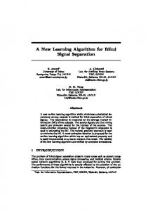
The proposed algorithm is compared with the following algorithms: • Conventional Negentropy stochastic gradient descent algorithm [1]: This algorithm is described by (5) with µ r suitably set to 0.0005. • Fast-ICA [2],[8]: this off-line algorithm as described by (6) presents a reference performance for the Negentropybased algorithms. It is presented to show how successful the separation algorithms can be in separating the original sources • Natural gradient based on Maximum likelihood (NAG): This on-line algorithm proposed by Amari [4], [5] converges much faster than stochastic gradient algorithms .It is considered as the reference on-line algorithm in the ICA domain. It is described by the following equation:
[
∑∑
which is supposed to be a permutation matrix at Wopt . The above cost function thus penalizes the deviation of P from the permutation structure. The first test used the 4 sources with a randomly generated mixing matrix presenting a rather difficult mixing situation: 0.7486 0.5624 0.3829 0.4798 0.3741 0.3723 0.2528 0.3683 (18) A= 0.4542 0.7928 0.3429 0.7646 0.7952 0.9678 0.3771 0.0386 The result of this first test is presented in Fig.1. It clearly shows the fast convergence rate of the proposed algorithm.
]
W = W + µ r I − f (y ) y T W (16) where µ r is set to 0.0005 and f (y ) is chosen to be 2 tanh (y ) [7], where y is the vector of all the outputs y i , i = 1L N . One advantage of the natural gradient algorithm is that it does not require pre-whitening. However, the algorithm estimates all the outputs at once and is suitable only for BSS. Failure to estimate the correct number of sources in advance or sudden changes in the number of sources may lead to illconditioned matrix situation. It is important to note that comparing the proposed algorithm with natural gradient algorithm could be a rather harsh judgment of the new algorithm. The on-line natural gradient algorithm serves only for blind signal separation. On the other hand, the proposed algorithm, serves for both blind signal separation and blind signal extraction. It estimates the data sequentially, in a deflationary manner. But this deflationary approach can also cause the accumulation of errors from the first estimated source to the following ones. In addition, the off-line algorithm implemented as in [8] is allowed to process the data in as many iterations as necessary until convergence is below a certain predetermined error, set to the power of 10-4. Despite these facts, simulation results show that the proposed algorithm
Figure 1 Cross-talking results for N=4 and a single run with the mixing matrix A as in (18)
The second test was to run each set of data (the 4 sources and the 10 sources) 100 times with different mixing
3
matrices stochastically generated. The data were prewhitened prior to the separation algorithm. Figures 2 and 3 present the results of this second test. Those figures representing the average performance of the different algorithms confirms that the proposed algorithm converges faster than the existing on-line Negentropy and the natural-gradient maximum likelihood algorithms, and proves its efficiency with different mixing situations. It is worth noting that the reference performance of the off-line Fast ICA algorithm is reached through 20 iterations on average for the 4 sources, and about 70-80 iterations for the 10 sources case.
V. CONCLUSION In this paper we introduced an improved on-line algorithm for blind signal separation using the Negentropy principle. The modifications implemented in (7)-(14) provide very good results confirmed by the assessment quality measure obtained for different mixtures. The algorithm actually not only improves over the existing on-line Negentropy-based algorithm, but it also exhibits superior performance when compared to the Natural gradient Maximum-Likelihood algorithm.
VI. REFERENCES [1] [2]
[3]
[4] [5]
[6] [7]
[8]
Figure 2 Cross-talking average result for N=4 and 100 runs with different mixing situations
[9]
Figure 3 Cross-talking average result for N=10 and 100 runs with different mixing situations
4
Hyvärinen A., Karhunen J. and Oja E, “Independent Component Analysis ", Haykin S., ed., John Wiley & Sons, 2001. Hyvärinen A. , “ Fast and Robust Fixed-point Algorithms for Independent Component Analysis”, IEEE Transactions Neural Networks, vol. 10, no. 3, pp. 626-634, 1999. Hyvärinen A. and Oja E. , “A Fast Fixed-Point Algorithm for Independent Component Analysis, Neural Computation, vol. 9, no. 7, pp. 1483-1492, 1997. Amari S., “Natural Gradient Works Efficiently in Learning", Neural Computation, vol. 10, pp. 251-276, 1998. Douglas S. C. and Amari S., “Natural Gradient Adaptation", Unsupervised Adaptive Filtering, Vol. I: Blind Source Separation, Haykin S., ed. New York: Wiley, 2000, pp. 13-61. Haykin S., ed. “Unsupervised Adaptive Filtering", Vol. I: Blind Source Separation, John Wiley & Sons, 2000. Benesty J., “An Introduction to Blind Source Separation of Speech Signals", Acoustic Signal Processing for Telecommunication, Gay S. and Benesty J., ed ,Kluwer Academic Publisher, 2000, pp. 321-329. Helsinki University of Technology, Laboratory of Computer and Information Science, Neural Network Research Center, “The FastICA Package for MATLAB" http://www.cis.hut.fi/projects/ica/fastica/ Helsinki University of Technology, Laboratory of Computer and Information Science, Neural Network Research Center, “ICA Link Collection" http://www.cis.hut.fi/projects/ica/book/links.html.