A RobustICA-Based Algorithm for Blind Separation of ... - arXiv

> REPLACE THIS LINE WITH YOUR PAPER IDENTIFICATION NUMBER (DOUBLE-CLICK HERE TO EDIT)
REPLACE THIS LINE WITH YOUR PAPER IDENTIFICATION NUMBER (DOUBLE-CLICK HERE TO EDIT) < characteristic of the source signals. In [22], [31], Authors studied the relationship between the number of frames of the STFT analysis and the BSS algorithms based on frequency framework. They argued the BSS algorithms in frequency domain are significantly affected by the number of the mixing matrices. Also in [22], [31], Authors proposed a method of applying the ICA adaptation to a group of frequencies in order to leave the size of the STFT large enough to achieve accurate separation processes. This method assumed that the acoustic propagation approximated is based on an anechoic model, i.e. as the DRR decreases. There are several drawbacks for separating the acoustic sources based on frequency domain methods [22], [40]. First of all, when we have a high reverberation environment, this requires us to increase the number of demixing matrices to ensure an efficient estimation for the source signals. However, this requirement is not easy to satisfy, especially if we have short observation signals of the source signals. Therefore, inspired by the works of V. Zarzoso,P. Comon [5], [6], this paper considers several challenges for the convolutive mixtures in the frequency domain in order to carry out the RobustICA-based algorithm in the frequency domain. We can summarize these challenges as follows.  Increasing the immunity of the BSS algorithm towards the outlets, e.g. signals’ length, additive noise, reverberation time and source moving etc.  Implementing should be optimized to be suitable for the real-time operation [42] in order to make the real-time DSP processor handle the computational cost without interruptions or distortions.  Effectively treating the scaling and permutation problems in the frequency domain.  Reducing the computational complexity of the ICA algorithms based on the frequency framework.  Controlling the accuracy of the ICA algorithm especially when short mixtures are available and the demixing matrices are not constrained by any anechoic model. Regarding the paper’s notation of matrix computation, a matrix is denoted as a bold capital letter such as , is the matrix transpose of , its Frobenius norm is marked by , an identity matrix of size n is denoted as , a vector is denoted as bold small letter such as , and scalars are denoted as a small letter such as . The remainder of the paper is organized as follows. Section II provides a brief description of convolutive mixtures and the problem statement. Section III presents the RobustICA-based method in the frequency domain. In Section IV, we perform solving the ambiguities in the ICA algorithm based on the frequency domain. The comparative experiments’ results and conclusions are given in Section V and Section VI, respectively.

2

II. CONVOLUTIVE MIXTURES A convolutive mixture can be considered a natural extension of the instantaneous BSS problem. Assume an dimensional vector of received discrete time signals is to be produced at time from an -dimensional vector of source signals , where , by using a stable mixture model [2]:

1.0

∑

2.0

∑

where represents the linear convolution operator and ( ) matrix of mixing coefficients at time-lag .

(1) is an

A. Problem Definition Assume that elements denote the coefficients of the Finite Impulse Response (FIR) filter and is the maximum unknown channel length. Then, the noise-free convolutive model is written as follows: ∑ (2) Thus, one can find an approximate inverse channel matrix in order to recover the source signals such that ∑ ̂ (3) where is the length of the inverse of the channel impulse response. There are two approaches to solve this problem and recover the source signals. Time domain approaches have several general drawbacks; for example, should be selected at least equal to the unknown true channel . Therefore, for a long mixing filter, which means long transfer functions, the computation will be too expensive [2], [14], [22]. Using the IIR filter instead of the long FIR filter to overcome this problem causes increased instability and might require inversion of the non-minimum phase filters [2], [3], [22]. Moreover, time approaches are sensitive to channel order mismatch [3]. That said, time domain methods are suitable and very efficient for small mixing filters such as in a communication channel [2], [12]. Because of all these limitations to time domain approaches, we focus our study on frequency domain approaches to solve the BSS problem. The main advantage of a frequency domain BSS approach is the ability to apply the set of any instantaneous ICA algorithms to solve the convolutive BSS problem. On the other hand, the main challenges of BSS in the frequency domain are permutation and scaling ambiguities. Refer to [1], [3], [22] for a recent survey. However, one can re-map the aforementioned BSS models into the frequency domain by applying the Discrete Fourier Transform (DFT) on the observed signals in order to transform it to the instantaneous mixtures problem as follows: (4)

> REPLACE THIS LINE WITH YOUR PAPER IDENTIFICATION NUMBER (DOUBLE-CLICK HERE TO EDIT) < where

is a frequency index, is a frame index, and . The previous equation is considered to be valid only for periodic signals . However, it is approximately valid if the time-convolution is circular. Therefore, ensuring that the time convolution is circular [1] requires making the Fourier Transform length significantly larger than the maximum length of the mixing channels [6]. In [28], [40], researchers imposed the spectral smoothing approach in order to mitigate the circularity effect in frequency domain BSS methods. In practice, to avoid the convergence into local minima during the separation processes, one can separate the observed signal at each frequency bin. Thus, the sampled observed signals are sampled at the discrete time instant using the sampling frequency . Then one can transform the sampled signals into time-frequency domain using the short time Fourier transform (STFT) applied to overlapped samples of the observed signals. However, one can express the time-frequency of the mth sensor at frame as follows ∑

(

) (5)

Where denotes the windowing function, here, we usually use the Hanning window since it is typically for acoustic signals. The Hanning window [17] is given by (

(

))

a half of the frequency bins symmetry property to find the others.

3

, and then use the

III. THE PRESENTED METHOD BASED ON THE ROBUSTICA FRAMEWORK

In this section, a new strategy is proposed, based on the RobustICA method of the kurtosis framework. Here, one needs to first recall the time-frequency representation of the observed vector equation (2), (16) The aim of this study is to estimate the demixing matrix from the observed vector under the assumption that the impulse response of all mixing filters is assumed constant during the recording. The estimated source vector is given as the following at each frequency bin: (17) A. Step1: Preprocessing (Data Whitening) In the preprocessing step, the demixing matrices are detected up to a unitary matrix using the second order statistic (SOS). This step was used to reduce the noise and to eliminate redundancy in the data at each frequency bin. The covariance matrix ( ) of the noise-free observed signals can be expressed by (18) By substituting

in (16), one gets

as follows

(6)

In a real-world scenario, we use the reverberation time to approximately define the length of the impulse response, since the impulse response functions are theoretically infinite. The reverberation time is the required time that reduces the energy of sounds into where the sound signal becomes no longer active or “dies away”. Therefore, the convolutive ICA model can be approximated into a series of the instantaneous ICA model as follows: (7) Where represents the frequency bin, denotes the time domain frame, e.g. in a short time frequency transform, is a column vector of the observed signals in frequency domain, is a column vector of the original source signals and is an mixing matrix in frequency domain. For the sake of simplicity, let us assume that the number of source signals is equal to the number of the observed signals , i.e., . Thus, by applying the ICA algorithm to the at each frequency bin, one can recover the estimated source signals as follows: (8) where is the demixing matrix at frequency bin. Also, due to the well-known symmetry property of the Fourier Transform, one can simply find demixing matrices ( ) as

(19) By imposing Tikhonov regularization techniques [47] to avoid the ill-posed problem, where it is well-known that regularization is an effective way to avoid the ill-conditioned matrix, the equation (19) becomes as follows: (20) Where

is

( (

an

identity

matrix,

)) it is regularization parameter with

and is

a positive constant and is a trace operator of the estimation covariance matrix . Note that the regularization method here just adds energy constraint in order to boost the covariance matrix to be a well-conditioned matrix. Therefore, the can be decomposed as (21) where

is a

matrix satisfying (22)

and

is an matrix

diagonal matrix. So, from (22), the will be (23)

where is a full rank unitary matrix and . However, the whitening step obtained matrix so that

> REPLACE THIS LINE WITH YOUR PAPER IDENTIFICATION NUMBER (DOUBLE-CLICK HERE TO EDIT) < the whitened data vector has covariance of identity matrix , which can be obtained as follows: (24) (25) The estimated source signals can be recovered with a linear Zero-Forcing (ZF) equalizer. Then the estimated source vector is (26) After the preprocessing step, the estimation of the source signals reduces to determining the unitary matrix (rotation matrix). B. Step 2: Determining the rotation matrix (unitary matrix) . One way of finding the rotational matrix is by maximizing the normalized fourth-order marginal cumulant (Kurtosis contrast) of the whitened data in (25). To estimate in (26), this paper exploits the statistical independence of the equalized source vector. More precisely, the unitary matrix will be estimated by utilizing the independent property of the estimated source vector at each frequency bin in the normalized fourth-order marginal cumulant of whitened data as follows: | ]

[|

[|

| ] | [

[|

| ]

]|

(27)

where represents the expectation operator. Based on the deflation approach to ICA [30], one can estimate the nth source signal as follows (28) where represents the conjugate-transpose operator, is the nth column vector of the demixing matrix and is nth source signal at each th frequency bin and qth frame time. According to [1], [2], the column vector of the demixing matrix can be estimated for all users due to the batch adaptation by a gradient decent method as follows (29) where denotes the iteration index, is the nth column vector of the demixing matrix at iteration and is the gradient of the contrast measure that updates the demixing vector in the demixing matrix . Gradient function depends on the cost function that ICA would maximize /minimize in order to extract the source signal [5]. Herein, this paper refers to the use of the ICA techniques based on the kurtosis criterion, which is given in (27), as follows: [|

| ]

[| |

| ] | [ |

]|

(30)

Having the RobustICA’s search-method of the kurtosis criterion in (30) in order to choose the optimal step size [6] as follows: | ( )| (31) where is the gradient of Kurtosis contrast . One can easily choose the optimal step size based on one of the algebraic methods instead of using the exact line search as in [13], [14] to avoid the intensive computation and other

4

limitations as in [6]. Therefore, it is easy to find the global optimum step size for the criteria that can be expressed as a polynomial function of due to its roots, e.g. the criteria kurtosis [6], the constant modulus [13] and the constant power [2]. Therefore, the RobustICA performs an optimal step-size of estimating the nth source signal, based on optimization, for lth iteration, th frequency bin, and th frame as follows: o Step1) initialize value for the weight vector o Step2) Compute the optimal step size polynomial coefficients. For Kurtosis contrast, the optimal step size polynomial is given by ∑ (32) where the coefficients can be obtained at each iteration by the observed signal block and the current values of and . Details can be found in [6]. o Step 3) Extract the optimal step size polynomial root . The root can be obtained by using the Ferrari’s formula as in [48]. o Step 4) Select the optimal step size polynomial root as follows | ( )| (33) o Step 5) Find the updated weighed vector (34) where is the nth gradient of Kurtosis contrast at lth iteration. o Step 6) Normalize and update the weight vector

‖

(35)

‖

where is a norm of . o Step 7) Go back to step 2 until the convergence. To prevent locking onto a previously extracted source, or when the old and new vectors are in the same direction, the learning converges and their absolute dotproduct value reaches close to 1. Thus, owning the deflation method proposed in [30] avoids different vectors from converging at the same maxima. However, each vector of { } needs to be orthogonalized before each iteration. Based on the Gram-Schmidt orthogonalization, the deflation scheme estimates each independent component at each iteration step. Gram-Schmidt orthogonalization of component can be expressed as follows ∑

( ‖

) ‖

(36) (37)

where a new weight vector is obtained by subtracting the vector projected from the old weight vector. The following steps summarize the presented algorithm procedure: o Start o Perform the time-frequency representation as in (4). o For each frequency bin o Pre-processing of the observed data and imposing the Tikhonov regularization parameter to avoid the ill-conditioning problem of the covariance matrix and to mitigate the performance degradation.

> REPLACE THIS LINE WITH YOUR PAPER IDENTIFICATION NUMBER (DOUBLE-CLICK HERE TO EDIT)
REPLACE THIS LINE WITH YOUR PAPER IDENTIFICATION NUMBER (DOUBLE-CLICK HERE TO EDIT) < The most common is based on the inter-frequency correlation of speech envelopes [33], [36]. The inter-frequency correlation technique exploits the nature of speech production, where it’s known that all spectral components of speech signals increase as the talker speaks louder. In that sense, several weighted techniques and criteria have been proposed to impose the frequency-coupling between the adjacent frequency bins. For more details, see [3], [22]. Although these techniques perform well in the simulations, they are not sophisticated when they are applied to a real recording room. They suffer from propagation error or delays. For example, if an error occurs at a certain frequency bin, it may increase the possibility that it will occur again at the following frequency bins. Therefore, in the literature [3], [22], [32], researchers avoid propagation error by estimating a frequencyindependent reference profile, which is called a centroid, due to using a clustering-based method for each separated source. They then structure the frequency-dependent profiles such that they are all matched with a different frequencyindependent reference profile at each frequency bin. The main steps of the clustering-based techniques are as follows:  Define the quantities that are used in the clustering, such as the signal envelopes of the source profiles, the log-power of the source profiles, etc.  Choose the measure that is used to determine the matching level between the centroids and the profiles, such as correlation, distance, etc.  Choose the cluster technique. In [21], [28], the profile of a separated signal is chosen as the envelope of the separated source where | |. In [22], Authors are chosen for the profile of a separated signal to be a certain dominance measure. Whereas, in [38], the profile of a separated signal is defined to be its centered log-power spectral density where the log-power profile is given as follows: [ ] (49) In clustering-based approaches, the length of the profiles is also an important parameter in terms of accuracy, especially for short signals. This work is essentially going to set up the profiles for the overlapping frames over the whole signal. Once we construct the profiles of the separated signals, then we compute the centroids in order to perform the clustering. The clustering-based technique is essentially based on the assumption that profiles coming from the same source at different frequency bins still have more match level than those coming from other sources. Actually, the most common methods to associate each source profile to a centroid at each frequency bin are based on 1) maximizing correlation measures [69], [70] and 2) minimizing distance measures across the factorial times of the possible permutations at each frequency bin [38]. However, authors employ the iterative techniques to update the centroids and the permutation matrices. In other words, they update the centroids first, and then they permute the source profiles to each desired centroid and match them together using one of

6

the two previous measures, i.e. distance [38] or correlation in [21], [28] and [31]. In spite of the fact that the aforementioned iterative methods perform well, they tend to be significantly more expensive in terms of cost and computational complexity since they have the factorial times of the possible permutations at each frequency bin. To avoid this drawback in the aforementioned iterative methods in [32], Nion et al. propose a more efficient modification of the clustering strategy, which is updating the whole permutation matrices and centroids simultaneously. In other words, the update of the centroids and permutation matrices are not interleaved. Thus, their modification has improved these iterative methods in terms of computational complexity. Their methods can be summarized as follows: Step 1. Determine the centroids and compute them. Consider the matrix that is structured from the profiles . One can extend the matrix to the matrix by concatenating the matrices . In order to enforce the profile points in matrix varying smoothly with time, we have to encounter the computation of the profiles for overlapping frames. Hereafter, we just need to classify these profile points into clusters due to applying the k-mean algorithm on the matrix to carry out a frequency-independent centroid matrix [ ] . The centroid matrix is structured by summing all the points within a cluster, which have attained a minimum distance regarding the centroid cluster. Step 2. Estimate the permutation matrices. In the previous step, we reduced the computational processes to find that the permutation matrix , subject to , matches the frequency-independent centroid matrix at each frequency bin. Therefore, one can choose to minimize the distance that is given in [38] as follows (50) Or one can chose the correlation criteria that is given by [21], [22] [31] as follows ∑ 〈 〉 (51) where 〈 〉 is the correlation coefficient. In terms of performance, the first group generally does better than the second group, especially at the small data sample available. But it is not optimal in a practical sense, since we don’t usually have geometric information about the real environmental conditions. In that sense, the second group performed better than first group, especially if we have a large sample set of data, because they are based on the clusteringbased techniques (i.e.: correlation, distance, etc.) and they are more robust to real-world scenarios. For more details, refer to [3] [22]. V. EXPERIMENTS’ RESULTS In this section, Monte Carlo Simulations are carried out. It

> REPLACE THIS LINE WITH YOUR PAPER IDENTIFICATION NUMBER (DOUBLE-CLICK HERE TO EDIT) < is assumed that the number of sources is equal to the number of observation “sensors”. The experiments have been carried out using the MATLAB software on an Intel Core i5 CPU 2.4GHz processor and 4G MB RAM. We examine the performance of the RobustICA-based algorithm developed in this paper. The time-frequency representation of the observed data is computed as explained in section II due to the ShortTime-Fourier-Transform. Then, for each frequency bin, we find the demixing matrix.We will solve the scale and permutation ambiguities based on the aforementioned techniques. To help explain this process, we divided this section into two subsections. First, we illustrate the performance of the RobustICA-based algorithm with different permutation methods in the literature [3], [22]. We study the effect of the type of the windows on the performance of the presented algorithm as well as the effect of overlapping parameter. Second, we provide the performance of the presented algorithm in two real-world scenarios that are generated in adverse conditions by F. Nesta, in [40], and compare it with other state-of-the-arts in [40], [20], and [34] and [38], labeled as “RR-ICA”, “IVA”, “Parra”, and “Pham”, respectively. In this paper, we evaluate the performance of the presented algorithm due to the BSS_EVAL toolbox, which is proposed in [49]. We use time-invariant filters of 1024 taps to represent the signal-to-interference ratio (SIR) and source-to-distortion ratio (SDR). A. Section 1 In this subsection, we study the computational complexity and the performance of the presented algorithm based on several criteria to solve the scale and permutation ambiguities in the frequency domain BSS problem. Let’s define these criteria as follows:  Method 1 is the RobustICA-based algorithm with clustering of envelope profiles with a distance measure iterative procedure [22], [31].  Method 2 is the RobustICA-based algorithm with clustering of log-power profiles with a correlation measure iterative procedure [22], [50].  Method 3 is the RobustICA-based algorithm with clustering of envelope profiles with a distance measure kmeans procedure [35], [32].  Method 4 is the RobustICA-based algorithm with clustering of log-power profiles with a correlation measure kmeans procedure [22], [32].  Method 5 is the RobustICA-based algorithm with clustering of dominance-profiles with a correlation measure iterative procedure [22].  Method6 is the RobustICA-based algorithm with clustering of dominance-profiles with a correlation measure iterative kmeans procedure [22], [32].

7

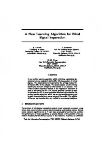
Fig. 1. Configuration of the two experimental setups that were conducted by Francesco Nesta1 in [40]:, a) room is characterized for Test1, b) classroom is characterized for Test2

In this section, we have used real world recordings, drawn from the experiments which were conducted in [40] named Test1. We would like to thank the authors who provided these recordings on their website “http://bssnesta.webatu.com/testhscma.html”. The two sources were recorded at with two microphones spaced apart to avoid spatial aliasing. The chosen room was characterized by a moderate reverberant time of . The room had dimensions of as shown in Fig. 1. The signal duration was fixed at 9 sec. 20 method 1

15

method 2

10

method 3 method 4

5

method 5 method 6

0 0.5s

1s

2s

4s

9s

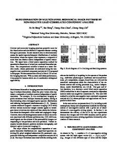
Fig. 2. Results obtained in Test1 experiments. The SIR performance of the presented algorithm with various permutation solvers

In fig. 2 and fig.3, we show the performance of the RobustICA-based algorithm with various aforementioned techniques of permutation solvers in terms of the SIR and SDR, respectively. In comparison, we notice that the dominance-profiles provide more robustness in terms of the signal’s length, although the envelope profiles are more sensitive to the signal’s length than the log-power profiles. Moreover, the dominance-profiles’ approach with the iterative procedure has the same performance as with the kmean procedure. Also, Fig.4 shows the corresponding CPU time of each permutation method that need to solve the permutation ambiguity.

> REPLACE THIS LINE WITH YOUR PAPER IDENTIFICATION NUMBER (DOUBLE-CLICK HERE TO EDIT)
REPLACE THIS LINE WITH YOUR PAPER IDENTIFICATION NUMBER (DOUBLE-CLICK HERE TO EDIT) < 20

9

15 proposed method

15

Proposed Method

10

RR-ICA

RR-ICA

10

IVA

5

IVA Parra's Mehtod

5

Parra's method

Pham's method

0 0.5

0 0.5

1

2

4

9

Fig. 7. Results obtained in the Test1 experiments. Best performance is reported in terms of SIR, by applying the given algorithms with different signal lengths

Fig 7 & 8 and 9 & 10, show the summary analysis of the presented algorithm versus other algorithms for the Test1 and Test2 configurations, respectively. These graphs report the best performance of each algorithm over the FFT size. Obviously, the RobustICA-based algorithm outperforms the other algorithms for any signal length in terms of SIR and SDR. Moreover, in Fig. 11, we illustrate the impact of the FFT length on the performance of the proposed algorithm in terms of SIR. Clearly, the presented algorithm performs well, especially during reasonable FFT length in regard to other corresponding algorithms as shown in Fig.11. Based on these results, one can show that the presented algorithm is stable in terms of the high reverberation environment and variations of the observations’ parameters. Furthermore, the presented algorithm performs well in terms of stability and speed convergence. Owning the optimal step size, deflation and regularization techniques makes the presented algorithm more robust and allows it to perform well even in adverse conditions.

1

2

4

9

pham's algorihtm

Fig. 9. Results obtained in the Test2 experiments. Best performance is reported in terms of SIR, by applying the given algorithms with different signal lengths

8 7 6 5 4 3 2 1 0

proposed method RR-ICA IVA Parra's method

0.5

1

2

4

9

pham's algorihtm

Fig. 10. Results obtained in the Test2 experiments. Best performance is reported in terms of SDR, by applying the given algorithms with different signal lengths

VI. CONCLUSION

This paper presented the RobustICA-based algorithm to solve the frequency-domain BSS problem for convolutive acoustic mixtures in several adverse conditions. Through the real-world experiments, we show the superiority of the presented algorithm among other popular algorithms in the 12 literature in terms of the performance and complexity computation. Moreover, we compared several permutation 10 solvers in terms of computation complexity and performance Proposed Method to provide the RobustICA-based algorithm with an efficient 8 frequency-dependent permutation scheme. Finally, we studied RR-ICA the effect of several parameters on the separation performance 6 IVA of the presented algorithm. We also presented the effect of the 4 type of the window on the separation performance and we also Parra's method showed that the performance improves at a certain range of pham's algorihtm 2 overlapping between the signals. Lastly, in this paper, we showed the performance of a system that can work efficiently 0 with around 0.5–10 seconds of input data, which is close to the 0.5 1 2 4 9 real-time implementation. Accordingly, the presented algorithm is optimized to be suitable for the real-time Fig. 8. Results obtained in the Test1 experiments. Best performance is reported in operation. As a result, it is suitable for a large number of terms of SDR, by applying the given algorithms with different signal lengths applications to ensure the real-time implementation.

> REPLACE THIS LINE WITH YOUR PAPER IDENTIFICATION NUMBER (DOUBLE-CLICK HERE TO EDIT) < 25 20

proposed method

15

RR-ICA

10

IVA

5

Parra's method

0

pham's algorihtm

Fig. 11. Impact of FFT length, 2-by-2 case, Results obtained in the Test2 experiments.

REFERENCES [1]

[2] [3]

[4]

[5]

[6]

[7]

[8]

[9] [10]

[11]

[12]

[13] [14]

[15]

[16]

[17]

P. Comon, C. Jutten (eds.), “Handbook of Blind Source Separation Independent Component Analysis and Applications.” (Academic Press, Oxford, 2010). A. Cichocki, S.-I. Amari, Adaptive Blind Signal and Image Processing: Learning Algorithms and Applications, John Wiley & Sons, Inc., 2002. M. S. Pedersen, J. Larsen, U. Kjems, and L. C. Parra, “A survey of convolutive blind source separation methods,” in Springer Handbook of Speech Processing. New York: Springer, 2007. A. Cichocki, R. Zdunek, S.-I. Amari, Nonnegative matrix and tensor factorizations: applications to exploratory multi-way analysis and Blind Source Separation, John Wiley & Sons, Inc., 2009. P. COMON, ``Independent Component Analysis, a new concept,'' Signal Processing, Elsevier, 36(3):287--314, April 1994PDF Special issue on Higher-Order Statistics. V. Zarzoso and P. Comon, “Robust Independent Component Analysis by Iterative Maximization of the Kurtosis Contrast with Algebraic Optimal Step Size,” IEEE Transactions on Neural Networks, vol. 21, no. 2, pp. 248–261, 2010. Hyvarinen. A, "Fast and robust fixed-point algorithm for independent component analysis". IEEE Transactions on Neural Network, vol. 10, no. 3, pp. 626–634, May 1999. Hyvarinen. A. E.Oja, "A fast fixed-point algorithm for independent component analysis,” Neural Computation, vol. 9, no. 7, pp. 1483–1492, 1997. F. Cardoso. On the performance of orthogonal source separation algorithms. In Proc. EUSIPCO, pages 776–779, 1994a. Jean-François Cardoso, “High-order contrasts for independent component analysis,” Neural Computation, vol. 11, no 1, pp. 157–192, Jan. 1999. A. Bell, T. J. Sejnowski, “An information-maximization approach to blind separation and blind deconvolution”, Neural Computation, 7:11291159, 1995. K. Waheed and F. Salem, “Blind information-theoretic multiuser detection algorithms for DS-CDMA and WCDMA downlink systems,” IEEE Trans. Neural Netw., vol. 16, no. 4, pp. 937–948, Jul. 2005. A.-J. van der Veen and A. Paulraj, “An analytical constant modulus algorithm,” IEEE Trans. Signal Process., vol. 44, pp. 1136– 1155, 1996. D. T. Pham and P. Garat, “Blind separation of mixture of independent sources through a quasi-maximum likelihood approach,” IEEE Trans. Signal Process, vol. 45, no. 7, pp. 1712–1725, Jul. 1997. B. A. Pearlmutter and L. C. Parra, “Maximum likelihood blind source separation: A context-sensitive generalization of ICA,” Adv. Neural Inf. Process. Syst., pp. 613–619, Dec. 1996. Fujisawa, H. and Eguchi, S. (2008). Robust parameter estimation with a small bias against heavy contamination. J. Multivariate Anal. 99 2053– 2081. S.C.Douglas, X.Sun, "Convolutive blind separation of speech mixtures using the natural gradient," Speech commun, vol. 39. pp. 65–78, (2002).

10

[18] Yoshioka, Takuya Nakatani, Tomohiro Miyoshi, Masato Okuno, Hiroshi G. "Blind Separation and Dereverberation of Speech Mixtures by Joint Optimization,” IEEE Transactions on Audio Speech and Language Processing, Volume. 19, Issue. 1, pp. 69, 2011. [19] A. Cichocki, R. Zdunek, S. Amari, G. Hori and K. Umeno, “Blind Signal Separation Method and System Using Modular and HierarchicalMultilayer Processing for Blind Multidimensional Decomposition, Identification, Separation or Extraction,” Patent pending, No. 2006124167, RIKEN, Japan, March 2006. [20] Intae Lee, Taesu Kim, and Te-Won Lee. Independent vector analysis for convolutive blind speech separation. In Blind Speech Separation. Springer, September 2007. [21] Solvang, Hiroko Kato Nagahara, Yuichi Araki, Shoko Sawada, Hiroshi Makino, Shoji "Frequency-Domain Pearson Distribution Approach for Independent Component Analysis (FD-Pearson-ICA) in Blind Source Separation,” IEEE Transactions on Audio Speech and Language Processing, Volume 17, Issue. 4, pp. 639, 2009. [22] H. Sawada, S. Araki, and S. Makino. Frequency-domain blind source separation. In Blind Speech Separation. Springer, September 2007. [23] Saruwatari, H. Kawamura, T. Nishikawa, T. Lee, A. Shikano, K. "Blind source separation based on a fast-convergence algorithm combining ICA and beamforming,” IEEE Transactions on Audio Speech and Language Processing, Volume 14, Issue 2, pp. 666, 2006. [24] Low, S.Y. Nordholm, S. Togneri, R. "Convolutive Blind Signal Separation With Post-Processing,” IEEE Transactions on Speech and Audio Processing, Volume 12, Issue 5, pp. 539, 2004. [25] F. Nest, P. Svaizer and M. Omologo “Convolutive BSS of short mixturesby ICA recursively regularized across frequencies", IEEETrans. Audio, Speech, Lang. Process., vol. 19, no. 3, pp.624 -639 2011 [26] S. C. Douglas and M. Gupta "Scaled natural gradient algorithms for instantaneous and convolutive blind source separation", Proc. ICASSP, vol. II, pp.637 -640 2007 [27] T. S. Wada and B.-H. Juang "Acoustic echo cancellation based on independent component analysis and integrated residual echo enhancement", Proc. WASPAA, pp.205 -208 2009 [28] H. Sawada , S. Araki , R. Mukai and S. Makino "Blind extraction of dominant target sources using ICA and time–frequency masking", IEEE Trans. Audio, Speech, Lang. Process., vol. 14, no. 6, pp.2165 -2173 2006 [29] S. Araki , S. Makino , T. Nishikawa and H. Saruwatari "Fundamental limitation of frequency domain blind source separation for convolutive mixture of speech", Proc. ICASSP, pp.2737 -2740 2001 [30] E. Ollila "The deflation-based fastICA estimator: Statistical analysis revisited", IEEE Trans. Signal Process., vol. 58, no. 3, pp.1527 -1541 2010 [31] H. Sawada, R. Mukai, S. Araki, and S. Makino, “A robust and precise method for solving the permutation problem of frequency-domainblind source separation,” IEEE Trans. Speech Audio Process., vol. 12, no. 5, pp. 530–538, Sep. 2004. [32] D. Nion , K. N. Mokios , N. D. Sidiropoulos and A. Potamianos "Batch and adaptive PARAFAC-based blind separation of convolutive speech mixtures", IEEE Trans. Audio, Speech Lang. Process., vol. 18, no. 6, pp.1193 -1207 2010 [33] K. Rahbar and J.-P. Reilly "A frequency domain method for blind source separation of convolutive audio mixtures", IEEE Trans. Speech Audio Process., vol. 13, no. 5, pp.832 -844 2005 [online] Available: http://www.ece.mcmaster.ca/~reilly/kamran/id18.htm [34] L. Parra and C. Spence "Convolutive blind separation of non-stationary sources", IEEE Trans. Speech Audio Process., vol. 8, no. 3, pp.320 327 2000 [online] Available: http://ida.first.fhg.de/~harmeli/download/download_convbss.html [35] C. Serviegrave;re and D.-T. Pham ”Permutation correction in the frequency domain in blind separation of speech mixtures", EURASIP J. Appl. Signal Process., no. 1, pp.1 -16 2006 [36] N. Mitianoudis and M. Davies”Audio source separation of convolutive mixtures", IEEE Trans. Speech Audio Process., vol. 11, no. 5, pp.489 497 2003 [37] A. Westner and J. V. M. Bove ”Blind separation of real world audio signals using overdetermined mixtures", Proc. ICA\'99, 1999 [online] Available: http://sound.media.mit.edu/ica-bench [38] D.-T. Pham, C. Servière and H. Boumaraf "Blind separation of convolutive audio mixtures using nonstationarity", Proc. Int. Workshop Indep. Compon. Anal. Blind Signal Separation (ICA\'03), pp.981 -986 2003

> REPLACE THIS LINE WITH YOUR PAPER IDENTIFICATION NUMBER (DOUBLE-CLICK HERE TO EDIT) < [39] F. Nesta, “Techniques for robust source separation and localization in adverse environment”, PhD thesis, University of Trento, April, 2010. [40] F. Nesta , P. Svaizer and M. Omologo "Convolutive BSS of short mixturesby ICA recursively regularized across frequencies", IEEETrans. Audio, Speech, Lang. Process., vol. 19, no. 3, pp.624 -639 2011 http://bssnesta.webatu.com/testhscma.html [41] Herbert Buchner, Robert Aichner, and Walter Kellermann. TRINICON: A versatile framework for multichannel blind signal processing. In Proceedings of IEEE International Conference on Acoustics, Speech and Signal Processing, volume 3, pages 889–892, Montreal, Canada, May 17-21 2004. [42] Robert Aichner, Herbert Buchner, Fei Yan, and Walter Kellermann. A real-time blind source separation scheme and its application to reverberant and noisy acoustic environments. Signal Process. 86(6):1260–1277, 2006. [43] Z. Koldovsky and P. Tichavsky. Time-domain blind audio source separation using advanced component clustering and reconstruction. In Proceedings of HSCMA, Trento, Italy, May 2008. [44] J.-T. Chien and H.-L. Hsieh “Nonstationary source separation using sequential and variational Bayesian learning", IEEE Trans. Neural Netw. Learn, Syst., vol. 24, no. 5, pp.681 -694 2013 [45] E. Vincent, S. Araki, and P. Bofill. The 2008 signal separation evaluation campaign: A community-based approach to large-scale evaluation. In ICA ’09: Proceedings of the 8th International Conference on Independent Component Analysis and Signal Separation, pages 734– 741, Berlin, Heidelberg, 2009. Springer-Verlag. [46] Takahashi, Yu. Saruwatari, H., Shikano, K., "Real-time implementation of blind spatial subtraction array for hands-free robot spoken dialogue system,” Intelligent Robots and Systems, 2008. IROS 2008. IEEE/RSJ International Conference on, On page(s): 1687–1692. [47] V. V. Vasin, “Some tendencies in the Tikhonov regularization of illposed problems,” J. Inverse and Ill-Posed Problems, vol. 14, no. 8, pp. 813-840, Dec. 2006. [48] W. H. Press, S. A. Teukolsky, W. T. Vetterling, and B. P. Flannery, Numerical Recipes in C. The Art of Scientific Computing, 2nd. Cambridge, UK: Cambridge University Press, 1992. [49] E. Vincent, C. Fevotte, and R. Gribonval. Performance measurement in blind audio source separation. IEEE Trans. Audio, Speech and Language Processing, 14(4):1462–1469, 2006. [50] M. Zibulevsky, “Blind source separation with relative Newton method,” in Proc. ICA 2003, 2003, pp. 897–902.

11