A New Online Secondary Path Modelling Method for Feedforward Active Noise Control Systems Pooya Davari and Hamid Hassanpour Department of Electrical and Computer Engineering, Mazandaran University, Shariatee Av, Babol, Iran,
[email protected] ,
[email protected]
Abstract- An Online secondary path modelling method using a white noise as a training signal is required in many applications of active noise control (ANC) to ensure convergence of the system. Not continually injection of white noise during system operation makes the system more desirable. The purposes of the proposed method are two folds: controlling white noise by preventing continually injection, and benefiting white noise with a larger variance. The modelling accuracy and the convergence rate increase when a white noise with larger variance is used, however larger the variance increases the residual noise, which decreases performance of the system. This paper proposes a new approach for online secondary path modelling in feedfoward ANC systems. The proposed algorithm uses the advantages of the white noise with larger variance to model the secondary path, but the injection is stopped at the optimum point to increase performance of the system. Comparative simulation results shown in this paper indicate effectiveness of the proposed approach in controlling active noise.
I.
INTRODUCTION
With the growth of industrial equipments such as: fans, engines, compressors, and transformers acoustic noises become a serious problem. Active noise control (ANC) is a technique that efficiently attenuates low frequencies unwanted noises where passive methods are either ineffective or tend to be very expensive or bulky. An ANC system is based on a destructive interference of an anti-noise with equal amplitude and opposite phase replica primary noise (the unwanted noise). Following the superposition principle, the result is cancellation or reduction of both noises [1]. The effect raised by the secondary path transfer function, the path leading from the noise controller output to the error sensor measuring the residual noise, generally causes instability to the standard least mean square (LMS) algorithm. In general FxLMS algorithm [1] is used to overcome the instability problem. The FxLMS algorithm uses estimation of the secondary path to reimburse the problem raised by the transfer function. In practical cases the secondary paths are usually time varying or non-linear, which leads to a poor performance or system instability. Therefore, online modelling of secondary path is required to ensure convergence of the ANC algorithm [2, 3, 4, 5]. Most of online secondary path modelling techniques entail injection of the additional random noise as a training signal to afford the felicitous estimation of the secondary path [1]. White noise is usually utilized as an ideal training signal in
978-1-4244-1706-3/08/$25.00 ©2008 IEEE.
modelling the secondary path [3, 4, 5]. White noise with larger variance improves modelling accuracy and convergence rate [5], nevertheless, with the cost of an increased residual noise. Thus, existing online secondary path modelling techniques use white noise with a low variance (usually 0.05 variance) to model the secondary path in order to sustain a low residual noise in steady state. The proposed system is based on an FxLMS algorithm as a main part of the system. The system uses a variable step size (VSS) LMS algorithm [4] to adapt the modelling filter of the secondary path. The proposed algorithm uses white noise with a large variance (as large as 0.8) in modelling the secondary path. However, to increase performance of the algorithm and to prevent the instability effect raised by the large variance white noise, the VSS-LMS algorithm is stopped at the optimum point. This increases noise attenuation and allows benefiting advantages of white noise with a larger variance. In addition, not having the white noise makes the system more desirable as continuous existence of the noise in the environment may have an unpleasant result. A sudden change in the secondary path leads to divergence of the online secondary path modelling filter. To abate this problem, the proposed algorithm is designed in the way that it controls the secondary path changes. A sudden change in secondary path during the operation makes the algorithm to reactivate injection of the white noise to modify the secondary path estimation. Common secondary path modelling methods use off-line estimation of the secondary path prior to online modelling [3, 4]. Off-line estimation can be obtained when the primary noise is absent. However, in many practical cases the primary noise exists even during the off-line modeling. This adversely affects the accuracy of the modeling filter. Therefore, the proposed method models the secondary path without the need of using off-line estimation of the secondary path. Considering the above features in the proposed method assists obtaining a better convergence rate and modelling accuracy, which results in a robust system. We show that this online estimation of the secondary path has no impact on the accuracy of the estimation. The organization of this paper is as follows. In section 2, the feedforward ANC system is briefly described. Section 3 introduces online secondary path modeling method and the proposed approach. In section 4, we illustrate our simulation results, and finally in Section five conclusions are drawn.
Fig. 1. Block diagram of feedforward ANC system using FxLMS algorithm.
III. ON LINE SECONDARY PATH MODELING METHOD
II. FEEDFORWARD ANC SYSTEM Transfer function of the secondary path has a crucial role in generating anti-noise in ANC applications as it is non-linear and introduces delay causing instability problem to the standard LMS algorithm. The instability problem can be resolved using the FxLMS algorithm [1] as it uses estimation of the secondary path. This algorithm can be applied to both feedback and feedforward structures. The block diagram of a feedforward FxLMS ANC system is shown in Fig. 1 [1]. Here, P(z) is the primary path, the acoustic response from the reference noise source to the error sensor; and S(z) represents the secondary path. In this figure, Sˆ ( z ) is estimation of the secondary path S(z). The secondary signal y(n) is generated as: y (n) = wT (n) x (n),
(1)
where w(n) and x(n) are the coefficient and signal vectors of length L, order of the FIR filter W(z), at time n. These coefficients are updated by the FxLMS algorithm as follows: wl (n + 1) = wl ( n) + μx′( n − 1)e( n)
(2) l = 0,1,..., L − 1 , μ > 0 ,
A. Existing Approaches The basic online secondary path modelling method which used random noise as a training signal (Fig. 2) was proposed by Eriksson et. al [6]. This method introduced another adaptive filter to model S(z) during online operation of ANC system. Several methods have later been proposed which could improve performance of the Eriksson’s method. Among the most recent online secondary path modelling methods [2][8], the method presented by Akhtar et. al [4] appears the best choice. Since the proposed method is based on Akhtar’s algorithm, here we briefly described this algorithm [4]. Consider Akhtar’s method [4] shown in Fig. 3. The residual error signal e(n) of this algorithm is expressed as:
e(n) = d ( n) − y′(n) + v′( n)
y ′( n) = s( n) ∗ y ( n) , v′(n ) = s (n ) ∗ v(n) ,
(3)
is the filtered reference signal. For a deep study on feedforward FxLMS algorithm the reader may refer to [1].
Fig. 2. Eriksson’s method [3] for ANC system with online secondary path modelling.
(4)
where v(n) is an internally generated white Gaussian noise, which is injected at the output of the control filter W(z). In this figure Sˆ ( z ) is the modelling FIR filter with length M that generates vˆ′(n) expressed below:
vˆ ′( n) = sˆ T (n)v M ( n) .
where μ is the step size, and xˆ ′(n) = Sˆ ( n) ∗ x( n) ,
Fig. 3. Akhtar’s method [4] for ANC system with online secondary path modelling.
(5)
As the figure shows, vˆ′(n) generates the error signal for both the modelling filter Sˆ ( z ) and the control filter W(z) by subtracting from e(n): (6) f (n) = [d (n) − y′(n) + v′(n)] − vˆ′(n) . Coefficients of the modelling filter Sˆ ( z ) are updated as follows: (7) sˆ(n + 1) = sˆ(n) + μ s (n) f (n)v(n) , where μ s (n) is the step-size parameter of the VSS-LMS algorithm which will be explained later. Finally coefficients of the control filter W(z) are updated as below: (9) w(n + 1) = w(n) + μ w (n) f (n) xˆ′(n) . The input to the LMS algorithm is derived by filtering the reference signal through Sˆ ( z ) : xˆ ′( n ) = sˆT ( n ) x M ( n ) ,
(10)
where xM (n) = [ x(n), x (n − 1),..., x(n − M + 1)]T is an M sample reference signal. The VSS-LMS algorithm is used to update modelling filter Sˆ ( z ) coefficients. For more detail on theory of this algorithm reader may refer to [4]. As we mentioned before, the modelling filter in equation (7) is updated using the step-size parameter ( μ s (n) ) of VSS-LMS algorithm and this parameter is calculated using the following three steps [4]: • Initially, the power of error signals e(n) and f(n) are computed: Pe (n ) = λPe ( n − 1) + (1 − λ )e 2 ( n)
Pf (n) = λPf (n − 1) + (1 − λ ) f 2 (n) . •
•
Then, the ratio of the estimated powers is obtained: ρ (n) = Pf (n) / Pe (n) .
ρ (0) ≈ 1 , limn → ∞ ρ (n) → 0 Finally, the step size is calculated as follows: μ s (n) = ρ (n) μ s min + (1 − ρ (n))μ s max ,
where μ s min , μ s max and λ
Fig. 4. Block diagram of the proposed feedforward ANC system.
(11)
(12)
(13)
are experimentally determined.
Using VSS-LMS algorithm increases the modelling accuracy and correspondingly improves system performance. Indeed, Akhtar’s method completely provided these features. B. Proposed Method As mentioned before, preventing continuous injection of white noise during system operation makes the system more desirable and increased noise attenuation. The main purpose of the proposed method is to control white noise by preventing continually injection to improve the system performance. This ability makes the system to benefit the large variance white noise and to overcome its disadvantages. White noise with larger variance results in a better modelling accuracy and convergence rate [5]. However, larger the variance increases the residual noise, which decreases performance of the system. Existing online secondary path modelling techniques [2]-[8] control the secondary path changes during system operation by continuous injection of white noise. Thus, these methods use white noise with a low variance to model the secondary path in order to maintain a lower residual noise in steady state. To use the advantage of large variance white noise and to adapt the system for secondary path changes, we propose a new system on the basis of Akhtar’s method [4]. The proposed method modifies the Akhtar’s algorithm to achieve a higher system performance. Fig. 4 shows block diagram of the proposed ANC system. To increase performance of the algorithm and to prevent the disadvantages of the white noise, the VSS-LMS algorithm is stopped at the optimum point. This increases noise attenuation and allows benefiting the advantages of white noise with a large variance. Here, the VSS-LMS algorithm is briefly described to show the way the optimum point is obtained. The VSS-LMS algorithm is initially set to a small step size. During the process of this
algorithm, μ s is increased as the error signal f(n) decreases and vice versa. It needs to be noted that any increase of the step size corresponds to a faster convergence of the adaptive algorithm. Consequently, once W(z) is slow in reducing e(n), the step size remains small which results in a lower convergence rate. Hence, the modeling filter, Sˆ ( z ) , converges to a good estimation when f(n) decreases. This happens when μ s increases as high as μ s max . Thus, the injection of the white noise is stopped at the optimum point which is measured using: (14) μ s max − μ s < α , 1 × 10 −5 < α ≤ 1 × 10 −3 . As can be seen from Fig. 4, this condition validity is monitored at the performance monitoring stage. By setting α to a lower value, the modelling error as well as the convergence rate is decreased, which results in an accurate modelling of the secondary path. In some practical cases the secondary path may suddenly change. This event derives system to diverge. To prevent this effect, Sˆ ( z ) needs to be updated. The proposed algorithm is design in such a way that it can monitor the secondary path changes by the following expression: 20 log10 f (n) < 0 .
(15)
If the validity of the above equation does not satisfy, the system reactivates the VSS-LMS algorithm and injects white noise to remodel Sˆ ( z ) . The same as before, the injection is stopped at the optimum point using (14). The above procedure is repeated during the system operation to adapt the algorithm with characteristics of the environment. As can be seen, the proposed algorithm controls the white noise injection by using (14) and (15), which results in a high performance system. Estimation of the secondary path can be obtained by using the off-line modeling method followed by an online modeling. However, as mentioned before, in some applications the primary noise exists even during the off-line modeling in which adversely affects the accuracy of the modeling filter. Therefore, with the advantages of the large variance white noise, there is no need of using off-line estimation of the secondary path in the proposed approach as it is required in the existing methods [3,4].
The parameters for Eriksson’s method are adjusted as μ w = 5 × 10 −4 and μ s = 1 × 10 −2 . These parameters are exactly set following [4], and for the proposed method we set
α to 1.65 ×10 −4 . To show the convergence rate and modelling accuracy of the system we use relative modelling error defined as below:
(a)
M −1 2½ ° ¦ [ si ( n) − sˆi ( n)] ° ° ° ΔS (dB ) = 10 log10 ® i = 0 M −1 ¾ 2 ° ° ¦ [ si ( n)] °¿ °¯ i=0
(16)
To signify performance of the system on noise reduction the following equation is used: 2 § · ¸ R = −10 log10 ¨¨ ¦ e (n) 2 ¦ d ( n) ¸¹ ©
(17)
The larger the positive value of R indicates that the more noise reduction is achieved. All the results shown in these cases are averaged on 10 experiments. (b) Fig. 5. Magnitude response of the acoustic paths (Solid line: Original path, Dashed line: Changed path at n=20,000): (a) Magnitude response of the primary path P(z), (b) Magnitude response of the secondary path S(z).
IV. SIMULATIONS RESULTS and PERFORMANCE EVALUATION
In this section the proposed ANC system is simulated using Matlab version 7.1. In this simulation, we have used the primary path P(z) and secondary path S(z) of the experimental data provided in [9]. The impulse responses of the primary and secondary paths are shown in Fig. 5. Using these data, P(z) and S(z) are considered as FIR filters with tap–weight lengths 48 and 16 respectively. Rate of the sampling frequency in this simulation was 2KHz. Comprehensive experiments have been performed to find appropriate values for a fast and stable performance of the ANC system. Length of FIR filter Sˆ ( z ) for modelling the secondary path, and length of the adaptive filter W(z) used for the noise cancellation have been chosen 16 and 32, respectively. In this simulations performance of the proposed method is compared with that of Akhtar’s [4] and Eriksson’s method [6]. We have performed simulations for two separate cases. We have performed simulations for three separate cases. In Case1, performance of the proposed method is evaluated in using both low and large variance white noises. Case2 shows the advantage of using a large variance white noise. Finally Case3 indicates effectiveness of the proposed algorithm in maintaining its performance against sudden changes of the acoustic paths behaviour. In these Cases the reference noise is a narrowband signal comprising frequencies of 100, 200, 300, and 400 Hz. Its variance is adjusted to 2, and a white noise with SNR of 30 dB is added. The parameters for the proposed method and Akhtar’s method are adjusted as μ w = 5 × 10 −4 , μ smin = 75 × 10 −4 , μ smax = 25 × 10−3 and λ = 0.99 .
A. Case1 Here we show the effect of controlling the injection of white noise during operation. In this case we compared the proposed approach with Akhtar’s method. Both methods evaluated under the situations defined in [4] using white noise with two different variances. To set the initial value for Sˆ ( z ) ( sˆ(0) ), offline secondary path modeling is performed. The off-line modeling is stopped when the modeling error (16) has been reduced to -5 dB.
(a)
(b) Fig. 6. Performance comparison between proposed method and the other existing methods: (a) Noise reduction achieved by white noise with variance of 0.05, (b) Noise reduction achieved by white noise with variance of 0.8.
Fig. 7. Modeling error versus iteration time n.
Fig. 8. Noise reduction versus iteration time n.
Fig. 6a shows that before proposed algorithm reached to the optimum point both plots are stick together, but after stopping the injection of the white noise at the optimum point proposed algorithm plot suddenly changed its path. As can be seen comparing with the other method the proposed method obtain more noise reduction. As Fig. 6b shows, the proposed method achieves a higher performance in using a larger variance white noise, in contradict, performance of two other methods is reduced by increasing the white noise variance. This is due to the non-stopping injection of white noise during the operation. B. Case2 As mentioned before, using offline estimation prior to online modeling procedure may cause problems for ANC system. Not using offline estimation decreases convergence rate and may affect on modeling accuracy. Using white noise with a large variance in secondary path modeling compensates these problems. As can be resulted from Case1, the proposed system not only eliminates the disadvantages of the large variance white noise but also benefits from its advantages. In this case, the proposed method is evaluated in terms of modeling accuracy and noise reduction, and the results are compared with the other methods. We use offline estimation (described in Case1) and white noise with variance 0.05 for the other methods. The proposed method uses white noise with variance 0.8 without using offline estimation. The comparative results are illustrated using (16) and (17) in Fig. 7 and 8. As can be seen, the proposed method, without using offline estimation, achieved a better performance compared to two other methods. C. Case3 In this case, it is assumed that both the primary and the secondary paths transfer functions are suddenly changed during the operation. Fig. 5 shows the magnitude response of the original and changed path. In this figure, the solid line represents the secondary path at start point, n = 0, and the dashed line represents the changed path at iteration n = 20000. Both methods are set under the condition described in [4], except that the proposed method is evaluated using white noise with variance 0.8.
(a)
(b) Fig. 9. Simulation results. (a) Relative modeling error versus iteration time n, (b) Modeling filter step size versus iteration time n.
Fig. 10. Noise reduction versus iteration time n.
The modeling error (16) and modeling filter step size are shown in Fig. 9, and the noise reduction (17) is shown in Fig. 10. As can be seen the proposed method maintains its performance with higher convergence rate. The importance is that the proposed method achieves a higher noise reduction (R) and convergence rate compared to the other methods. V. CONCLUSIONS This paper proposed a new method for online secondary path modelling in ANC systems. Computer simulations have been conducted for a single-channel feedforward ANC system. Simulation results demonstrated that the proposed method achieves a higher convergence rate, a more accurate modelling accuracy, and a better noise reduction performance compared with the existing approach. Eliminating continuous injection of the white noise and not initially using off-line secondary path estimation makes the proposed method more desirable for practical ANC systems. REFERENCE [1] [2]
[3]
[4]
[5]
[6]
[7]
[8]
[9]
S. M. Kuo and D. R. Morgan, “Active noise control: a tutorial review,” Proc. IEEE, vol. 8, no. 6, pp. 943–973, Jun. 1999. S. M. Kuo, and D. Vijayan,“A secondary path modeling technique for active noise control systems,” IEEE Trans. Speech Audio Processing, vol. 5, no. 4, pp. 374–377, 1997. M. T. Akhtar, M. Abe, and M. Kawamata, “Modified-filtered-x LMS algorithm based active noise control system with improved online secondary path modeling,” in Proc. IEEE 2004 Intern. Mid. Symp. Circuits Systems (MWSCAS2004), Hiroshima, Japan, July 25–28, 2004, pp. I-13–I-16. M. T. Akhtar, M. Abe, and M. Kawamata, “A Method for Online Secondary Path Modeling in Active Noise Control Systems,” in Proc. IEEE 2005 Intern. Symp. Circuits Systems (ISCAS2005), May 23–26, pp. I-264–I-267, 2005. Sen M. Kuo and Dipa Vijayan, “Optimized Secondary Path Modeling Technique for Active Noise Control Systems,” in Proc. IEEE AsiaPacific Conf. on Circuits and Systems, Taipei, Taiwan, pp. 370-375, 1994. L. J. Eriksson, and M. C. Allie, “Use of random noise for on-line transducer modeling in an adaptive active attenuation system,” J. Acoust. Soc. Am., vol. 85, issue 2, pp. 797–802, 1989. M. Zhang, H. Lan, and W. Ser, “Cross-updated active noise control system with online secondary path modeling,” IEEE Trans. Speech, Audio Proc., vol. 9, no. 5, pp. 598–602, 2001. C. Bao, P. Sas, and H. V. Brussel, “Adaptive active control of noise in 3-D reverberant enclosure,” J. Sound Vibr., vol. 161, no. 3, pp. 501– 514, 1993. S. M. Kuo, and D. R. Morgan, Active Noise Control SystemsAlgorithms and DSP Implementation. New York: Wiley, 1996.