A New Repair Operator for Multi-objective Evolutionary Algorithm in ...

A New Repair Operator for Multi-objective Evolutionary Algorithm in Constrained Optimization Problems Zhun Fan

Wenji Li

Xinye Cai

Guangdong Provincial Key Laboratory of Digital Signal and Image Processing Department of Electronic Engineering Shantou University, Guangdong, P.R. China

Department of Electronic Engineering Shantou University, Guangdong, P.R. China

College of Computer Science and Technology, Nanjing University of Aeronautics and Astronautics, Jiangsu, P.R. China

[email protected]

[email protected]

[email protected] Huibiao Lin Department of Electronic Engineering Shantou University, Guangdong, P.R. China

Shuxiang Xie

Erik Goodman

Department of Electronic Engineering Shantou University, Guangdong, P.R. China

BEACON Center for the Study of Evolution in Action, Michigan State University, East Lansing, MI, USA

[email protected]

[email protected]

[email protected]

ABSTRACT In this paper, we design a set of multi-objective constrained optimization problems (MCOPs) and propose a new repair operator to address them. The proposed repair operator is used to fix the solutions that violate the box constraints. More specifically, it employs a reversed correction strategy that can effectively avoid the population falling into local optimum. In addition, we integrate the proposed repair operator into two classical multiobjective evolutionary algorithms MOEA/D and NSGA-II. The proposed repair operator is compared with other two kinds of commonly used repair operators on benchmark problems CTPs and MCOPs. The experiment results demonstrate that our proposed approach is very effective in terms of convergence and diversity.

min F ( x)  ( f1 ( x), f 2 ( x), , f m ( x));   s.t. gi ( x)  0, i  1, 2, , q  h j ( x)  0, j  1, 2, p 

Where x  ( x1 , x2 ,

(1)

, xn )  R n is n-dimensional design

variables, F ( x)  ( f1 ( x), f 2 ( x),

, f m ( x))  R m is m-dimensional

objective vector. gi ( x)  0 define q inequality constraints, h j ( x)  0 define p equality constraints.

1. INTRODUCTION

The existing multi-objective constrained evolutionary algorithms combine the multi-objective evolutionary algorithms with the mechanisms of constraint handling [1]. At present, NSGA-II [2] and MOEA/D [3] are the two classical multi-objective evolutionary algorithms representing two categories of fitness assignment methods, namely fitness assignment based on domination and decomposition. In fitness assignment based on domination, the fitness is decided by non-dominated sorting and crowding distance. Representative algorithms using this type of fitness assignment method include MOGA [4] , PAES-II [5] , SPEA-II [6] and NSGA-II [2]. In fitness assignment based on decomposition, comparison and sorting of individuals are made via aggregation function with weights allocated specifically to all individuals. Typical algorithms of this category include IMMOGLS [7], UGA [8] , cMOGA [9] , MOGLS [10] , and MOEA/D [3].

Multi-objective optimization problems (MOPs) consist of more than one objectives, which are usually conflicting with each other. In other words, improvements in one objective may lead to the degradation of other objectives. It is impossible to make all of the objectives to be optimal at the same time. Instead, a set of solutions that represent the trade-off between multiple objectives exist for MOPs. In addition, different types of constraints are often unavoidable in MOPs. Such MOPs with constraints are usually termed multi-objective constrained optimization problem. Constraints can be roughly divided into two categories, equality and inequality constraints. Without loss of generality, a multiobjective constrained optimization problem can be defined as follows.

The existing constraints handling mechanism can be divided into four categories. They are feasibility maintenance, penalty function, separation of constraint violation and objective value and multiobjective evolutionary algorithms (MOEAs). The methods of feasibility maintenance are usually applied to the discrete optimization problems, such as the job shop scheduling problems and the vehicle routing problems. They either design appropriate coding and decoding methods to ensure that the individuals are feasible, or apply some mechanisms to repair the infeasible individuals. The main idea of penalty function method is adding one penalty term to the objective functions and transforming the constrained optimization problem into an unconstrained one. Typical methods of this category include segregated penalty

Categories and Subject Descriptors G.1.6 [Optimization]: Constrained optimization

General Terms Algorithms

Keywords Repair operators, Multi-objective constrained optimization

functions [17], death penalty functions [18], co-evolutionary penalty functions [19] and adaptive penalty functions [20] [21]. The mechanism of separation of constraint violation and objective value treats the objective and constraints separately. Typical methods of this category include stochastic ranking (SR) [11], infeasible driven evolutionary algorithm (IDEA) [12] and constraint dominate principle (CDP) [13]. The main feature of MOEAs is to transform a multi-objective constrained optimization problem to another multi-objective optimization problem with an additional objective, which regards the constraint condition as another objective and uses the existing MOEAs to optimize the transformed problem. Typical methods of this category include COMOGA [14], CW [15] and ATMES [16]. It is noteworthy that the penalty function method needs to tune the punishment factor, and the MOEAs method brings additional objective. In this paper, CDP method is used to handle constraints, which requires no additional parameters.

share the same constraint conditions. In terms of objective functions, we adopt ZDT test problems [28] but make some changes. In addition, nine ellipses are established in the objective space as the constraint conditions. The general form of constraint conditions are as follows: C ( x)  (( f1 (x)  cx )  cos( )  ( f 2 (x)  c y )  sin( )) 2 / a 2

 (( f1 (x)  cx )  sin( )  ( f 2 (x)  c y )  cos( )) 2 / b 2  1

(3)

The constraint C ( x) has five parameters ( , a, b, cx and c y ) , which can be used to further adjust the difficulty levels of the constraint conditions as needed. Among them  denotes the counterclockwise rotation angle of the ellipse. a and b control the lengths of the long axis and minor axis of the ellipse respectively.

cx and c y are two vectors representing the centers of the ellipses.

The remainder of the paper is organized as follows. Section 2 designs a set of multi-objective constrained optimization problems (MCOPs). Section 3 introduces the repair operator. Section 4 gives the experimental results of the CTP and MCOP optimization problems, and Section 5 concludes the paper.

For example, if we define the following parameters:

2. DESIGN OF MCOPs

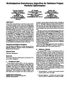
The distribution of constraining ellipses in the objective space is shown in Figure 1.

The existing multi-objective constrained optimization problems mainly consist of CTP [22][23] and CF[24]. CTP benchmark problems can be defined as follows: minimize f1 ( x)  x1  minimize f 2 ( x)  g (1  f1 / g ) 10   2 (2)  g ( x)  1  9 ( xi  10cos(2 xi )  10) i2  s.t. C ( x)  cos( )( f 2 ( x)  e)  sin( ) f1 ( x)   a | sin(b (sin( )( f 2 (x)  e)  cos( ) f1 (x)) c ) |d  

It is important to note that the problem can be made harder by setting g ( x) function with various local extreme. The inequality constraint C(x) has six parameters ( ,a,b,c,d,and e) . In fact, the above problem can be used as a constrained test problem generator by tuning these six parameters. Deb et al designed seven benchmark problems named CTP2-CTP8 by setting those six parameters. The original CTP2-CTP8 instances have only 2 decision variables and they are easy to solve. Hence, we extend the CTP2-CTP8 problems to ten decision variables and variable bounds are given by 0  x  1, i  1, i

 cx   0 1 0 1 2 0 1 2 3  c      y  1.5 0.5 2.5 1.5 0.5 3.5 2.5 1.5 0.5 a 2  0.1, b 2  0.2,  0.25

Figure 1. The distribution of constraint functions. Combining the constraint functions with objective functions, we design seven multi-objective constraint optimization problems, namely MCOP1-MCOP7. The objective functions of them are listed in Table 1. Table 1. Objective functions of MCOP1-MCOP7. Function Name

,10 . The six constraint

parameters are the same as those used in [22]. According to the final report on CEC’09 MOEA competition, MOEA/D and NSGA-II are not quite suitable for solving CF instances. Even though it is very easy to search feasible solutions for CF, finding the true Pareto front turns out to be very difficult. This paper mainly focuses on applying the repair operators in the framework of MOEA/D and NSGA-II. Because CF is not a suitable test suite for MOEA/D and NSGA-II, we design a new set of multi-objective constrained optimization problems (MCOPs) to validate the proposed repair operator in the framework of MOEA/D and NSGA-II. Unlike CTP2-CTP8 instances which have the same multi-objectives and each problem has different constraint conditions by selecting six different parameters, we design a set of problems that have different multi-objectives but

(4)

MCOP1 PF convex

MCOP2 PF discrete

Function Definition

minimize f1 ( x)  g  x1  minimize f 2 ( x)  g (1  f1 / g )  m   g ( x)  1  9 xi / ( m  1) i2   m x   30, [0,1] i 

minimize f1 ( x)  g  x1 minimize f ( x)  g (1  ( f / g ) 2 ) 2 1   m   g ( x)  1  9 xi / ( m  1) i2  m 30, x [0,1]    i 

minimize f1 ( x)  x1  minimize f 2 ( x)  g (1  f1 / g )    f1 sin(10 f1 )  m  0.25  g ( x)  1  9(( xi / ( m  1)) ) i2   m  10, xi  [0,1]

MCOP3 PF discrete

In order to facilitate discussion, we denote the formula (5) and formula (6) as Repair-A and Repair-B respectively. In this paper, we propose a new repair operator denoted as Repair-C. The formula of our proposed repair operator can be defined as follows:  U j ,if xi , j  L j xi , j     L j ,if xi , j  U j

minimize f1 ( x)  g  x1  minimize f 2 ( x)  g (1  f1 / g )  m  2  g ( x)  1  10(m  1)   ( xi  10cos(4 xi )) i 2    m  10, xi  [0,1]

MCOP4 PF convex

minimize f1 ( x)  g  x1 minimize f ( x)  g (1  ( f / g ) 2 ) 2 1   m  2  g ( x)  1  10(m  1)   ( xi  10cos(4 xi )) i2   m  10, xi  [0,1]

MCOP5 PF discrete

minimize f1 ( x)  1  exp(4 x1 )sin 6 (6 x1 )  minimize f 2 ( x)  g (1  ( f1 / g ) 2 )   m  2  g ( x)  1  10(m  1)   ( xi  10cos(4 xi )) i2  m  10, xi  [0,1] 

MCOP6 PF discrete

minimize f1 ( x)  1  exp(4 x1 )sin 6 (6 x1 )  minimize f 2 ( x)  g (1  f1 / g )  m  2  g ( x)  1  10(m  1)   ( xi  10cos(4 xi )) i 2    m  10, xi  [0,1]

MCOP7 PF convex

3. REPAIR OPERATOR Repair operators are used to fix the infeasible solutions that violate the box constraints. A lot of research concentrates on repairing the infeasible solutions for discrete multi-objective constrained optimization problems. However, very few researchers have paid attention to the repair operators for continuous multi-objective constrained optimization problems. At present, there are two commonly used repair operators. One of the most commonly used repair operator can be defined as follows:   L j ,if xi , j  L j xi , j    U j ,if xi , j  U j

(5)

Where xi , j represents the value of j-th component of individual i.

(7)

This repair operator is inspired in part by the concept of opposition-based learning (OBL) originally introduced by Tizhoosh [29]. The main idea of OBL is, for finding a better candidate solution, simultaneous consideration of an estimate and its corresponding opposite estimate has a potential to help search towards the global optimum in a more efficient way, due to an arguably better preservation of diversity in the searching population. For example, the differential evolution process can be defined as follows: xi , j  xi , j  F ( xr1, j  xr 2, j )

(8)

Where r1 and r2 are two unequal random integers and not equal to i . F denotes the factor of differential evolution, here we set F  0.5 . If xi , j is less than its lower bound L j , it can be inferred

that xi , j has a higher probability of getting a value close to its

lower bound L j . In this case if we fix xi , j to its upper bound U j ,

which can be approximately considered as an opposite estimate of xi , j , then this operator has a potential to increase the diversity of the population according to the philosophy of OBL. Even though this choice is a bit counterintuitive because normally people think fixing xi , j to its lower bound L j is a better choice,

but we shall also not ignore the possibility that fixing xi , j to its lower bound L j , which is a value with a lot loss of potential after many previous search attempts, the search may have a higher likelihood to be stuck in local minima. To verify this hypothesis, we conduct a lot of experiments which are described in detail in the Section of Experimental Study.

4. EXPERIMENTAL STUDY 4.1 Experimental Settings In order to evaluate the performance of repair operators mentioned in section 3, we combined these three repair operators with NSGA-II and MOEA/D and then studied the experimental results on CTP2-CTP8 and MCOP1-MCOP7. Thirty independent runs with the six algorithms are conducted. The detailed parameter settings of these six algorithms are summarized as follows.

variables. U j denotes the upper bound of j-th component of the

1) Setting for reproduction operators: The mutation probability Pm = 1/n (n is the number of decision variables) and its distribution index is set to be 20. For the DE operator, we set CR = 1.0 and F = 0.5 as recommended in [27].

decision variables.

2) Population size: N = 200.

Another commonly used repair operator proposed by Wang etc. [26] can be defined as follows:

3) Number of runs and stopping condition: Each algorithm runs 30 times independently on each test problems. The algorithm stops until 500 000 function evaluations.

L j denotes the lower bound of j-th component of the decision

  min{U j ,2 L j  xi , j },if xi , j  L j xi , j    max{L j ,2U j  xi , j },if xi , j  U j

(6)

4) Neighborhood size: T = 20.

5) Probability use to select in the neighborhood:   0.9 .

6) The maximal number of solutions replaced by a child： nr  2 .

4.2 Performance Metric In this work, performance of a constrained multi-objective evolutionary algorithm is evaluated in two aspects – convergence and distribution. Convergence describes the closeness of the obtained Pareto front to the true Pareto front. Distribution on the other hand depicts how the solutions in the obtained Pareto are distributed. We select two metrics - inverted generation distance (IGD)[30] and hypervolume (HV)[30]. Detailed definitions of them are given as follows: Inverted Generational Distance (IGD): Let p* is the ideal Pareto front set, A is an approximate Pareto front set achieved by evolutionary multi-objective algorithm. IGD metric denotes the distance between p* and A. It is defined as follows:

  y P d ( y , A)  IGD( P* , A)  | P* |      m     ( yi  yi ) 2    d ( y , A)  min y A  1 i     

(8)

Where m is the number of objectives, |P| denotes the size of set P , d ( y , A) denotes the minimum Euclidean distance between y* and A. IGD metric can reflects the convergence and diversity simultaneously. The smaller IGD metric means the better performance. Hypervolume (HV): HV simultaneously considers the distribution of the obtained Pareto front A and its vicinity to the true Pareto front. HV is defined as the volume enclosed by A and the reference vector r  (r1, r2 , , rm ) . HV can be defined as:

HV ( P) 

iP

vol (i)

(9)

Here, vol (i) represents the volume enclosed by solution i  A and the reference vector r . The maximum value of each objective in the ideal Pareto front set gives the value of each dimension of the reference point r , and thus constructs the reference point.

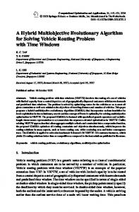
4.3 Experimental Result In order to demonstrate the effectiveness of the proposed repair operator, we first compared it with the other two repair operators Operator_A and Operator_B (discussed in section III) in the framework of MOEA/D-CDP on CTP2-CTP8 and MCOP1MCOP7 problems. The final populations with the best hypervolume metric in 30 independent runs with the three repair operators are shown in Figure 2.

Figure 2. The final populations with the best hypervolume metric in 30 independent runs

From Figure 2, it is clear that MOEA/D-Repair-C has obtained best Pareto fronts on CTP3, CTP7, MCOP5, MCOP6 and MCOP7. For CTP2, CTP5 and MCOP4, MOEA/D-Repair-A and MOEA/D-Repair-C have a similar Pareto front, which is better than the Pareto front obtained by MOEA/D-Repair-B. MOEA/DRepair-B and MOEA/D-Repair-C have a better Pareto front than MOEA/D-Repair-A on CTP4. For CTP6, CTP8, MCOP1, MCOP2 and MCOP3, the three methods have similar Pareto fronts. Overall MOEA/D-Repair-C outperforms or is at least competitive with MOEA/D-Repair-A and MOEA/D-Repair-B in all test cases. Table 2. IGD values of MOEA/D-Repair-A and MOEA/DRepair-B Instance

MOEA/D-Repair-A

MOEA/D-Repair-B

-

Mean

Std.

Mean

Std.

CTP2

6.81E-02

3.86E-02

1.46E-01

7.84E-02

CTP3

1.63E-01

9.45E-02

3.37E-01

1.71E-01

CTP4

4.68E-01

2.21E-01

5.88E-01

4.67E-01

CTP5

8.08E-02

3.70E-02

1.38E-01

9.20E-02

CTP6

1.29E-02

9.65E-03

1.28E-01

7.51E-02

CTP7

1.17E-01

4.86E-02

1.58E-01

7.13E-02

CTP8

3.77E-02

5.80E-02

2.72E-01

1.06E-01

MCOP1

2.39E-04

2.33E-06

2.40E-04

3.84E-06

MCOP2

2.56E-04

1.47E-07

2.56E-04

1.71E-07

MCOP3

2.71E-04

4.94E-07

2.71E-04

1.82E-06

MCOP4

8.96E-02

3.01E-02

1.21E-01

2.85E-02

MCOP5

1.67E-01

6.14E-02

2.88E-01

9.92E-02

MCOP6

1.03E-01

2.05E-02

1.23E-01

2.47E-02

MCOP7

1.09E-01

3.09E-02

1.28E-01

3.80E-02

Table 3. IGD values of MOEA/D-Repair-A and MOEA/DRepair-C Instance

MOEA/D-Repair-A

MOEA/D-Repair-C

-

Mean

Std.

Mean

Std.

CTP2

6.81E-02

3.86E-02

1.70E-04

3.15E-06

CTP3

1.63E-01

9.45E-02

1.40E-03

1.71E-04

CTP4

4.68E-01

2.21E-01

4.41E-02

2.83E-02

CTP5

8.08E-02

3.70E-02

6.85E-03

3.88E-03

CTP6

1.29E-02

9.65E-03

5.04E-04

1.99E-05

CTP7

1.17E-01

4.86E-02

1.39E-04

2.77E-07

CTP8

3.77E-02

5.80E-02

1.12E-03

1.32E-04

MCOP1

2.39E-04

2.33E-06

2.37E-04

3.68E-06

MCOP2

2.56E-04

1.47E-07

2.56E-04

4.65E-07

MCOP3

2.71E-04

4.94E-07

2.71E-04

3.03E-06

MCOP4

8.96E-02

3.01E-02

1.55E-02

1.62E-02

MCOP5

1.67E-01

6.14E-02

3.27E-02

3.49E-02

MCOP6

1.03E-01

2.05E-02

2.89E-02

2.08E-02

MCOP7

1.09E-01

3.09E-02

4.63E-02

1.60E-02

Table 4. T-test values of IGD among MOEA/D-Repair-A, MOEA/D-Repair-B and MOEA/D-Repair-C Instance

Repair-C vs Repair-A

Repair-C vs Repair-B

h-value

p-value

h-value

p-value

CTP2

1.00E+00

5.66E-14

1.00E+00

8.11E-15

CTP3

1.00E+00

1.53E-13

1.00E+00

8.79E-16

CTP4

1.00E+00

3.64E-15

1.00E+00

1.67E-08

CTP5

1.00E+00

6.17E-16

1.00E+00

7.15E-11

CTP6

-

1.00E+00

1.20E-09

1.00E+00

2.41E-13

CTP7

1.00E+00

2.36E-19

1.00E+00

8.56E-18

CTP8

1.00E+00

5.13E-04

1.00E+00

1.47E-20

MCOP1

1.00E+00

1.91E-02

1.00E+00

1.62E-03

MCOP2

0.00E+00

9.80E-01

0.00E+00

9.82E-01

MCOP3

0.00E+00

8.17E-01

0.00E+00

8.92E-01

MCOP4

1.00E+00

1.78E-17

1.00E+00

2.37E-25

MCOP5

1.00E+00

3.71E-15

1.00E+00

1.55E-19

MCOP6

1.00E+00

2.42E-20

1.00E+00

4.34E-23

MCOP7

1.00E+00

2.41E-14

1.00E+00

5.67E-16

Table 2 and Table 3 present the average values of IGD over 30 independent runs in the framework of MOEA/D. Table 4 presents the t-test values of IGD among three different repair operators. It can be observed that MOEA/D-Repair-C performs significantly better than other two methods on all the instances except for MCOP2 and MCOP3, and almost the same as the other two kinds of repair operators on MCOP2 and MCOP3 (with slightly bigger standard deviation). The main cause is that MCOP2 and MCOP3 (actually including MCOP1) are relatively easy to solve that the three different repair operators can not reflect differences on them. Table 5. HV values of MOEA/D-Repair-A and MOEA/DRepair-B HV -

MOEA/D-Repair-A

MOEA/D-Repair-B

CTP2

Mean 5.00E-02

Std. 1.02E-01

Mean 9.76E-03

Std. 3.71E-02

CTP3

3.83E-02

6.45E-02

0.00E+00

0.00E+00

CTP4

8.43E-03

3.21E-02

3.84E-02

8.43E-02

CTP5

2.16E-02

7.48E-02

1.83E-02

4.75E-02

CTP6

4.04E-01

8.34E-02

1.14E-01

1.89E-01

CTP7

2.43E-03

5.53E-03

9.74E-04

3.71E-03

CTP8

3.08E-01

1.40E-01

5.59E-02

1.46E-01

MCOP1

6.64E-01

1.78E-05

6.64E-01

2.05E-05

MCOP2

2.21E-01

8.54E-06

2.21E-01

1.50E-05

MCOP3

5.16E-01

3.43E-06

5.15E-01

2.23E-05

MCOP4

3.37E-02

1.22E-01

2.53E-04

9.64E-04

MCOP5

3.55E-03

1.40E-02

0.00E+00

0.00E+00

MCOP6

0.00E+00

0.00E+00

0.00E+00

0.00E+00

MCOP7

0.00E+00

0.00E+00

0.00E+00

0.00E+00

Table 6. HV values of MOEA/D-Repair-A and MOEA/DRepair-C Instance -

MOEA/D-Repair-A

MOEA/D-Repair-C

CTP2

Mean 5.00E-02

Std. 1.02E-01

Mean 4.77E-01

Std. 9.83E-05

CTP3

3.83E-02

6.45E-02

4.45E-01

1.90E-03

CTP4

8.43E-03

3.21E-02

3.08E-01

8.97E-02

CTP6

1.08E-02

7.22E-03

8.48E-02

7.72E-02

CTP5

2.16E-02

7.48E-02

2.52E-01

1.03E-01

CTP7

7.86E-02

4.44E-02

1.61E-01

8.43E-02

CTP6

4.04E-01

8.34E-02

4.99E-01

2.21E-04

CTP8

1.98E-02

9.15E-03

1.61E-01

1.47E-01

CTP7

2.43E-03

5.53E-03

5.46E-01

2.56E-05

MCOP1

2.74E-04

1.83E-05

4.52E-04

4.21E-05

CTP8

3.08E-01

1.40E-01

4.41E-01

4.72E-04

MCOP2

1.07E-02

2.04E-02

1.60E-02

1.05E-02

MCOP1

6.64E-01

1.78E-05

6.64E-01

6.06E-05

MCOP3

1.18E-04

4.38E-06

2.57E-04

4.12E-05

MCOP2

2.21E-01

8.54E-06

2.21E-01

4.60E-05

MCOP4

1.01E-01

3.14E-02

1.36E-01

6.00E-02

MCOP3

5.16E-01

3.43E-06

5.15E-01

2.98E-05

MCOP5

2.27E-01

8.64E-02

3.36E-01

1.05E-01

MCOP4

3.37E-02

1.22E-01

4.93E-01

1.70E-01

MCOP6

1.02E-01

4.07E-02

1.57E-01

5.35E-02

MCOP5

3.55E-03

1.40E-02

1.14E-01

1.09E-01

MCOP7

1.13E-01

3.51E-02

1.70E-01

4.87E-02

MCOP6

0.00E+00

0.00E+00

5.90E-02

1.02E-01

MCOP7

0.00E+00

0.00E+00

4.22E-02

1.20E-01

Table 7. T-test values of HV among MOEA/D-Repair-A, MOEA/D-Repair-B and MOEA/D-Repair-C Instance

Repair-C vs Repair-A

Repair-C vs Repair-B

Table 9. IGD values of NSGAII-Repair-A and NSGAII-Repair-C Instance -

NSGAII-Repair-A

NSGAII-Repair-C

CTP2

Mean 4.66E-02

Std. 3.23E-02

Mean 1.13E-04

Std. 4.49E-05

CTP3

1.03E-01

6.32E-02

2.95E-03

9.83E-04

CTP4

2.90E-01

1.67E-01

7.46E-02

2.32E-02

CTP5

6.14E-02

2.32E-02

1.01E-02

4.84E-03

CTP6

1.08E-02

7.22E-03

3.02E-04

1.16E-04

h-value

p-value

h-value

p-value

CTP2

1.00E+00

1.00E+00

1.23E-57

CTP3

1.00E+00

4.89E-31 1.12E-40

1.00E+00

4.07E-131

CTP4

1.00E+00

9.40E-25

1.00E+00

1.26E-17

CTP7

7.86E-02

4.44E-02

5.25E-05

1.54E-06

CTP5

1.00E+00

2.21E-14

1.00E+00

1.59E-16

CTP8

1.98E-02

9.15E-03

5.05E-04

8.50E-05

CTP6

1.00E+00

3.21E-08

1.00E+00

2.39E-16

MCOP1

2.74E-04

1.83E-05

7.20E-03

1.61E-02

CTP7

1.00E+00

2.77E-109

1.00E+00

1.97E-119

MCOP2

1.07E-02

2.04E-02

2.56E-02

2.14E-02

CTP8

1.00E+00

1.16E-06

1.00E+00

3.15E-21

MCOP3

1.18E-04

4.38E-06

1.45E-02

1.80E-02

MCOP1

0.00E+00

1.00E+00

0.00E+00

1.00E+00

MCOP4

1.01E-01

3.14E-02

2.72E-04

1.75E-05

MCOP2

0.00E+00

1.00E+00

0.00E+00

1.00E+00

MCOP5

2.27E-01

8.64E-02

1.83E-04

1.54E-05

MCOP3

0.00E+00

1.00E+00

0.00E+00

1.00E+00

MCOP6

1.02E-01

4.07E-02

4.31E-05

1.03E-05

MCOP4

1.00E+00

1.12E-17

1.00E+00

4.46E-23

MCOP7

1.13E-01

3.51E-02

9.72E-05

1.92E-05

MCOP5

1.00E+00

3.85E-07

1.00E+00

1.65E-07

MCOP6

1.00E+00

1.19E-03

1.00E+00

1.19E-03

MCOP7

1.00E+00

2.97E-02

1.00E+00

2.97E-02

-

Table 5 and Table 6 present the average values of HV over 30 independent runs in the framework of MOEA/D. Table 7 presents the t-test values of HV among three repair operators. From Table 5, Table 6 and Table 7, it can be observed that MOEA/D-RepairC performs significantly better than the other two kinds of methods on all the instances except for MCOP1, MCOP2 and MCOP3, which means that our proposed repair operator can effectively avoid the population falling into local optimum in the framework of MOEA/D. For MCOP1, MCOP2 and MCOP3, the three methods obtain almost the same results. Table 8. IGD values of NSGAII-Repair-A and NSGAII-Repair-B Instance -

NSGAII-Repair-A Mean

NSGAII-Repair-B Mean 1.17E-01

Std. 6.41E-02

Table 10. T-test values of IGD among NSGAII-Repair-A, NSGAII-Repair-B and NSGAII-Repair-C Instance

Repair-C vs Repair-A

Repair-C vs Repair-B

h-value

p-value

h-value

p-value

CTP2

1.00E+00

4.90E-11

1.00E+00

1.89E-14

CTP3

-

1.00E+00

2.07E-12

1.00E+00

3.82E-17

CTP4

1.00E+00

1.39E-09

1.00E+00

4.31E-13

CTP5

1.00E+00

2.00E-17

1.00E+00

6.34E-16

CTP6

1.00E+00

3.86E-11

1.00E+00

6.92E-08

CTP7

1.00E+00

5.03E-14

1.00E+00

2.61E-15

CTP8

1.00E+00

5.44E-17

1.00E+00

8.16E-08

MCOP1

0.00E+00

9.89E-01

0.00E+00

9.87E-01

MCOP2

0.00E+00

9.96E-01

0.00E+00

9.84E-01

MCOP3

0.00E+00

1.00E+00

0.00E+00

1.00E+00

CTP2

4.66E-02

Std. 3.23E-02

CTP3

1.03E-01

6.32E-02

3.12E-01

1.45E-01

MCOP4

1.00E+00

3.48E-25

1.00E+00

2.90E-18

CTP4

2.90E-01

1.67E-01

6.18E-01

3.26E-01

MCOP5

1.00E+00

4.03E-21

1.00E+00

3.36E-25

CTP5

6.14E-02

2.32E-02

1.12E-01

5.13E-02

MCOP6

1.00E+00

4.30E-20

1.00E+00

2.54E-23

MCOP7

1.00E+00

2.60E-25

1.00E+00

5.48E-27

Table 8 and table 9 present the average values of IGD over 30 independent runs in the framework of NSGA-II. Table 10 presents the t-test values of IGD among the three repair operators. It can be observed that similar to the results obtained in the framework of MOEA/D, the Repair-C performs better than Repair-A and Repair-B on all the instances except for MCOP1, MCOP2 and MCOP3. For MCOP1, MCOP2 and MCOP3, the three methods obtain almost the same results.

CTP3

1.00E+00

6.17E-28

1.00E+00

4.80E-55

CTP4

1.00E+00

1.52E-07

1.00E+00

5.41E-17

CTP5

1.00E+00

3.72E-12

1.00E+00

2.87E-14

CTP6

1.00E+00

2.94E-09

1.00E+00

2.69E-12

CTP7

1.00E+00

3.84E-28

1.00E+00

1.67E-36

1.00E+00

4.47E-18

1.00E+00

2.47E-10

Table 11. HV values of NSGAII-Repair-A and NSGAII-Repair-B

MCOP1

0.00E+00

9.91E-01

0.00E+00

9.87E-01

NSGAII-Repair-B

MCOP2

0.00E+00

1.00E+00

0.00E+00

9.93E-01 1.00E+00

Instance -

NSGAII-Repair-A Mean

CTP8

Mean 2.42E-02

Std. 5.49E-02

0.00E+00

1.00E+00

0.00E+00

4.77E-01

Std. 1.01E-01

MCOP3

CTP2

MCOP4

1.00E+00

2.43E-94

1.00E+00

5.43E-59

CTP3

4.37E-01

7.15E-02

9.47E-03

3.61E-02

MCOP5

1.00E+00

1.64E-36

1.00E+00

2.72E-206

CTP4

3.43E-01

4.51E-02

8.42E-03

3.21E-02

MCOP6

1.00E+00

1.95E-23

1.00E+00

1.81E-236

CTP5

1.37E-01

2.29E-02

1.37E-02

4.19E-02

MCOP7

1.00E+00

1.67E-36

1.00E+00

6.88E-195

CTP6

5.00E-01

4.24E-01

1.82E-01

2.02E-01

CTP7

5.47E-01

4.14E-02

1.97E-02

9.96E-02

CTP8

4.45E-01

3.63E-01

1.80E-01

1.94E-01

MCOP1

6.64E-01

6.64E-01

6.59E-01

6.29E-04

MCOP2

2.21E-01

1.92E-01

1.27E-01

5.24E-02

MCOP3

5.17E-01

5.17E-01

5.10E-01

1.57E-03

MCOP4

2.63E-02

8.14E-03

1.15E-02

4.91E-02

MCOP5

2.21E-01

7.38E-03

0.00E+00

0.00E+00

MCOP6

2.38E-01

2.38E-02

0.00E+00

0.00E+00

5. CONCLUSION

MCOP7

5.48E-01

1.83E-02

0.00E+00

0.00E+00

This paper proposes a new repair operator which employs a reversed correction strategy to fix the solutions that violate the box-constraint. In order to validate its performance on convergence and diversity, a new set of constrained multiobjective optimization problems is designed, to complement the well-known CTP test suite. The performance of the proposed repair operator has been compared with the other two kinds of commonly used repair operators. Experimental results show that it outperforms the other repair operators in terms of convergence and diversity, based on the two classic frameworks of MOEA/D and NSGA-II. The future work includes combining the proposed repair operator with other state-of-the-art algorithms to further validate the repair operator and improve the performance of the algorithms, and testing them in real-world applications.

Table12. HV values of NSGAII-Repair-A and NSGAII-Repair-C Instance

NSGAII-Repair-a

NSGAII-Repair-c

CTP2

Mean 1.01E-01

Std. 1.45E-01

Mean 4.77E-01

Std. 5.21E-04

CTP3

7.15E-02

9.84E-02

4.31E-01

9.21E-03

CTP4

4.51E-02

7.97E-02

1.50E-01

5.88E-02

CTP5

2.29E-02

5.21E-02

1.54E-01

6.62E-02

CTP6

4.24E-01

6.14E-02

5.00E-01

8.20E-04

CTP7

4.14E-02

1.38E-01

5.47E-01

4.14E-05

CTP8

3.63E-01

3.61E-02

4.44E-01

2.12E-04

MCOP1

6.64E-01

5.97E-05

5.85E-01

1.78E-01

MCOP2

1.92E-01

3.45E-02

8.03E-02

8.81E-02

MCOP3

5.17E-01

2.29E-05

3.15E-01

2.08E-01

MCOP4

8.14E-03

1.21E-02

6.64E-01

1.91E-04

MCOP5

7.38E-03

4.04E-02

2.21E-01

4.78E-05

MCOP6

2.38E-02

7.26E-02

2.38E-01

1.55E-05

MCOP7

1.83E-02

1.00E-01

5.48E-01

1.86E-04

-

Table 13. T-test values of HV among NSGAII-Repair-A, NSGAII-Repair-B and NSGAII-Repair-C Instance CTP2

Repair-C vs Repair-A

Repair-C vs Repair-B

h-value

p-value

h-value

p-value

1.00E+00

7.84E-21

1.00E+00

3.56E-47

Table 11 and Table 12 present the average values of HV over 30 independent runs in the framework of NSGA-II. Table 13 presents the t-test values of HV among three repair operators. From Table 11, Table 12 and Table 13, it can be observed that NSGA-IIRepair-C performs significantly better than other two kinds of methods on all the instances except for MCOP1, MCOP2 and MCOP3. For MCOP1, MCOP2 and MCOP3, the three methods obtain almost the same results. It can be therefore concluded that the proposed repair operator can also work well in the framework of NSGA-II.

6. REFERENCES

 Y. Wang, Z.X. Cai, Y.R. Zhou, and C.X. Xiao, “Constrained optimization evolutionary algorithms,” Journal of Software,Vol.20,No.1,January 2009,pp.11-29  Deb K, Pratap A, Agarwal S, et al. A fast and elitist multiobjective genetic algorithm: NSGA-II[J]. Evolutionary Computation, IEEE Transactions on, 2002, 6(2): 182-197.  Zhang Q, Li H. MOEA/D: A multiobjective evolutionary algorithm based on decomposition [J]. Evolutionary Computation, IEEE Transactions on, 2007, 11(6): 712-731.  Fonseca C M, Fleming P J. Genetic Algorithms for Multiobjective Optimization: FormulationDiscussion and Generalization[C].ICGA. 1993, 93: 416-423.  Corne D W, Jerram N R, Knowles J D, et al. PESA-II: Region-based selection in evolutionary multiobjective

optimization[C].Proceedings of the Genetic and Evolutionary Computation Conference (GECCO’2001. 2001.

 Zitzler E, Laumanns M, Thiele L. SPEA2: Improving the Strength Pareto Evolutionary Algorithm [J]. 2001.

 Ishibuchi H, Murata T. A multi-objective genetic local search algorithm and its application to flowshop scheduling[J]. Systems, Man, and Cybernetics, Part C: Applications and Reviews, IEEE Transactions on, 1998, 28(3): 392-403.  Leung Y W, Wang Y. Multiobjective programming using uniform design and genetic algorithm [J]. Systems, Man, and Cybernetics, Part C: Applications and Reviews, IEEE Transactions on, 2000, 30(3): 293-304.  Murata T, Ishibuchi H, Gen M. Specification of genetic search directions in cellular multi-objective genetic algorithms[C]//Evolutionary Multi-Criterion Optimization. Springer Berlin Heidelberg, 2001: 82-95.  Jaszkiewicz A. On the performance of multiple-objective genetic local search on the 0/1 knapsack problem-A comparative experiment [J]. Evolutionary Computation, IEEE Transactions on, 2002, 6(4): 402-412.

 Runarsson T P, Yao X. Stochastic ranking for constrained evolutionary optimization [J]. Evolutionary Computation, IEEE Transactions on, 2000, 4(3): 284-294.  Ray T, Singh H K, Isaacs A, et al. Infeasibility driven evolutionary algorithm for constrained optimization[M]//Constraint-handling in evolutionary optimization. Springer Berlin Heidelberg, 2009: 145-165.

 Deb K. An efficient constraint handling method for genetic algorithms [J]. Computer methods in applied mechanics and engineering, 2000, 186(2): 311-338.  P.D. Surry, N.J. Radcliffe, The COMOGA method: Constrained optimisation by multiobjective genetic algorithms, Control Cybern. 26 (3) (1997).

 Cai Z, Wang Y. A multiobjective optimization-based evolutionary algorithm for constrained optimization [J]. Evolutionary Computation, IEEE Transactions on, 2006, 10(6): 658-675.

 Wang Y, Cai Z, Zhou Y, et al. An adaptive tradeoff model for constrained evolutionary optimization [J]. Evolutionary Computation, IEEE Transactions on, 2008, 12(1): 80-92.

 Le RRG, Knopf-Lenoir C, Haftka RT. A segregated genetic algorithm for constrained structural optimization. In: Eshelman LJ, ed. Proc. of the 6th Int’1 Conf. on Genetic Algorithms. San Francisco: Morgan Kaufman Publishers, 1995. 558-565.  Hoffmeister F, Sprave J. Problem-independent handling of constraints by use of metric penalty functions [J]. 1996.  Huang F, Wang L, He Q. An effective co-evolutionary differential evolution for constrained optimization [J].

Applied Mathematics and computation, 2007, 186(1): 340356.

 Ben Hamida S, Schoenauer M. ASCHEA: new results using adaptive segregational constraint handling[C]//Evolutionary Computation, 2002. CEC'02. Proceedings of the 2002 Congress on. IEEE, 2002, 1: 884-889.  Coit D W, Smith A E, Tate D M. Adaptive penalty methods for genetic optimization of constrained combinatorial problems[J]. INFORMS Journal on Computing, 1996, 8(2): 173-182.  K. Deb, Multi-Objective Optimization using Evolutionary Algorithms.John Wiley & Sons, Ltd, Chichester, 2001.

 ]K. Deb, A. Pratap, and T. Meyarivan, “Constrained test problems for multi-objective evolutionary optimization,” In Proceedings of the First International Conference on Evolutionary Multi-Criterion Optimization (EMO-2001). Zürich, Switzerland, pp. 284-298, 2001.

 Zhang Q, Zhou A, Zhao S, et al. Multiobjective optimization test instances for the CEC 2009 special session and competition[J]. University of Essex, Colchester, UK and Nanyang Technological University, Singapore, Special Session on Performance Assessment of Multi-Objective Optimization Algorithms, Technical Report, 2008.  Zitzler E, Deb K, Thiele L. Comparison of multiobjective evolutionary algorithms: Empirical results [J]. Evolutionary computation, 2000, 8(2): 173-195.  Wang Y, Cai Z, Zhang Q. Differential evolution with composite trial vector generation strategies and control parameters [J]. Evolutionary Computation, IEEE Transactions on, 2011, 15(1): 55-66.

 H. Li and Q. Zhang, “Multiobjective optimization problems with complicated Pareto sets, MOEA/D and NSGA-II,” IEEE Trans. Evol. Comput.,vol. 13, no. 2, pp. 284–302, Apr. 2009.  Deb K. Multi-objective genetic algorithms: Problem difficulties and construction of test problems [J]. Evolutionary computation, 1999, 7(3): 205-230.

 Tizhoosh H R. Opposition-Based Learning: A New Scheme for Machine Intelligence[C]//CIMCA/IAWTIC. 2005: 695701.

 Bosman P A N, Thierens D. The balance between proximity and diversity in multiobjective evolutionary algorithms[J]. Evolutionary Computation, IEEE Transactions on, 2003, 7(2): 174-188.  Zitzler E, Thiele L. Multiobjective evolutionary algorithms: a comparative case study and the strength Pareto approach[J]. evolutionary computation, IEEE transactions on, 1999, 3(4): 257-271.