Hindawi Publishing Corporation Mathematical Problems in Engineering Volume 2015, Article ID 145258, 13 pages http://dx.doi.org/10.1155/2015/145258
Research Article A New Six-Parameter Model Based on Chebyshev Polynomials for Solar Cells Shu-xian Lun,1 Jing-shu Sang,2 and Ting-ting Guo2 1
College of New Energy, Bohai University, Jinzhou 121013, China School of Mathematics and Physics, Bohai University, Jinzhou 121013, China
2
Correspondence should be addressed to Shu-xian Lun;
[email protected] Received 29 December 2014; Accepted 2 April 2015 Academic Editor: Georgios Veronis Copyright © 2015 Shu-xian Lun et al. This is an open access article distributed under the Creative Commons Attribution License, which permits unrestricted use, distribution, and reproduction in any medium, provided the original work is properly cited. This paper presents a new current-voltage (I-V) model for solar cells. It has been proved that series resistance of a solar cell is related to temperature. However, the existing five-parameter model ignores the temperature dependence of series resistance and then only accurately predicts the performance of monocrystalline silicon solar cells. Therefore, this paper uses Chebyshev polynomials to describe the relationship between series resistance and temperature. This makes a new parameter called temperature coefficient for series resistance introduced into the single-diode model. Then, a new six-parameter model for solar cells is established in this paper. This new model can improve the accuracy of the traditional single-diode model and reflect the temperature dependence of series resistance. To validate the accuracy of the six-parameter model in this paper, five kinds of silicon solar cells with different technology types, that is, monocrystalline silicon, polycrystalline silicon, thin film silicon, and tripe-junction amorphous silicon, are tested at different irradiance and temperature conditions. Experiment results show that the six-parameter model proposed in this paper is an I-V model with moderate computational complexity and high precision.
1. Introduction Photovoltaic (PV) power generation system directly converts solar energy into electrical energy by using PV arrays. To obtain higher energy efficiency, PV power generation systems need to establish their simulation models to get optimized parameters. PV power generation system is mainly composed of PV arrays, controller [1–3], and inverter [4–6]. PV arrays, the core devices of PV power generation system, usually consist of solar cells in series and/or in parallel. There are two kinds of popular simulation models for solar cells, that is, the single-diode model and the double-diode model [7– 10]. Because of having fewer parameters, the single-diode model is simpler than the double-diode model. This makes the single-diode model widely used. Some efforts have been made to improve the accuracy of the single-diode model. According to the number of parameters, there are mainly three kinds of models, that is, the four-parameter model, the five-parameter model, and the seven-parameter model. The four-parameter model in [11] includes ideality factor, diode reverse saturation current, light-generated current,
series resistance. The four-parameter model has the fewest cell parameters, and then its expression is the simplest. However, the predicted accuracy of the four-parameter model is very limited. And the four-parameter model is validated only for monocrystalline silicon modules. On the basis of the four-parameter model, the five-parameter models are obtained by introducing shunt resistance [11–21]. The fiveparameter models are more precise than the four-parameter model in [11]. Compromising the number of parameters and the approximate accuracy, the five-parameter models are the most commonly used. The five-parameter models proposed in [11, 19–21] utilize the reciprocals of the slopes at the open-circuit point and short-circuit point to calculate the cell parameters. The two slope values are not usually provided by the manufacturers’ datasheet. And they can be obtained by using enough data pairs of experimental 𝐼-𝑉 characteristic under the certain condition. This makes it very complicated to obtain the slope values. Therefore, these five-parameter models actually have seven parameters rather than five parameters. The five-parameter model in [12] does not utilize the above-mentioned two slope parameters
2
Mathematical Problems in Engineering Rs
IL
ID
Ish
I
V
Rsh
RL
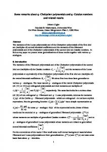
Figure 1: Single diode model.
and can accurately predict the performance of monocrystalline and polycrystalline silicon modules. However, the fiveparameter model in [12] exists large modeling errors for amorphous silicon solar cells. This may be due to the facts that series resistance in [12] is assumed to be a constant and the temperature dependence of series resistance is ignored. Here, temperature refers to the temperature of solar cells. The seven-parameter models proposed in [13, 22] add two additional parameters on the basis of the five-parameter model. For example, in [13], the two additional parameters are temperature coefficient for series resistance and the diode reverse saturation current radiation dependence, respectively. Temperature coefficient for series resistance describes the temperature dependence of series resistance. The value of series resistance changes exponentially with the cell temperature. The diode reverse saturation current radiation dependence describes the influence of irradiance on diode reverse saturation current, which is obtained by using the current and the voltage at maximum power point under the irradiance of 200 W/m2 and the temperature of 25∘ C. The extraction process for this parameter is very complicated. Although the seven-parameter model in [13] provides a more accurate 𝐼-𝑉 characteristic model, it is not widely used because of the complexity of parameter extraction. Therefore, we propose a new six-parameter model. In this paper, Chebyshev polynomials are developed to describe the relationship between series resistance and temperature. This makes a new parameter called temperature coefficient for series resistance introduced into the singlediode model. Therefore, the single-diode model has six cell parameters in this paper, that is, ideality factor, lightgenerated current, diode reverse saturation current, series resistance, shunt resistance, and temperature coefficient for series resistance. The new six-parameter model provides a simpler and more reasonable expression for series resistance and accurately predicts 𝐼-𝑉 characteristic for silicon solar cells. Five kinds of silicon solar cells with four different technology types, that is, monocrystalline silicon, polycrystalline silicon, thin film silicon and triple-junction amorphous silicon, are tested to validate the six-parameter model in this paper.
2. The Single-Diode Model of Solar Cells A solar cell is essentially a very large area p-n junction diode. Under illumination, a single-diode model of a solar cell can
be described by an equivalent circuit, shown in Figure 1. The 𝐼-𝑉 equation of a single-diode model is shown as follows: 𝐼 = 𝐼𝐿 − 𝐼𝑜 [exp (
𝑉 + 𝐼𝑅𝑠 𝑉 + 𝐼𝑅𝑠 , ) − 1] − 𝑎 𝑅sh
(1)
where 𝐼𝐿 (A) is light-generated current, 𝐼𝑜 (A) is diode reverse saturation current, 𝑅sh (Ω) is shunt resistance, and 𝑅𝑠 (Ω) is series resistance, 𝑎 is ideality factor which is defined as follows: 𝑎 = 𝑁𝑠 𝑛𝐼 𝑉𝑡 ,
(2)
where 𝑁𝑠 is the number of solar cells in series in a PV module, 𝑛𝐼 is diode ideality factor, and 𝑉𝑡 is thermal voltage which is defined as follows: 𝑉𝑡 =
𝑘𝑇 , 𝑞
(3)
where 𝑘 is Boltzmann’s constant (1.38066𝐸 − 23 J/K), 𝑇 (K) is cell temperature, and 𝑞 is electron charge (1.60218𝐸 − 19 C).
3. Chebyshev Polynomials Are Used to Model Series Resistance in the Six-Parameter Model Temperature dependence of series resistance has been quantitatively analyzed and various expressions are obtained [18, 21, 23–27]. Most of the expressions are nonlinear and implicit formulations about temperature. In [18, 21, 24], the relationship between series resistance and temperature is expressed as the exponential function of temperature. In [25], series resistance is literally expressed as the linear function of temperature. In fact, the expression also contains other electrical parameters at the same time, such as the short-circuit current and the voltage and the current at maximum power point, which are closely related to temperature. Therefore, the expression of series resistance in [25] is actually complex nonlinear. In addition, [13, 27] have given explicit representation of series resistance about temperature. Reference [27] has proved that series resistance of a solar cell belongs to positive temperature coefficient type. However, some of the series resistance of solar cells monotonically increases with the increase of temperature [23], but some of the series resistance of solar cells monotonically decreases with the increase of temperature [28, 29]. Therefore, for different kinds of solar
Mathematical Problems in Engineering
3
cells, the expression in [27] for temperature dependence of series resistance is limited. As is known, the expression of 𝐼-𝑉 characteristic is a transcendental equation and series resistance is an exponential function of temperature. When series resistance with the exponential function is substituted into 𝐼-𝑉 characteristic model, the processes of 𝐼-𝑉 characteristic modeling and parameter extraction will become complex and have computational burden. Therefore, in this paper, we follow the relationship between series resistance and temperature in [13] to develop a new expression of series resistance about temperature. Chebyshev polynomials are used to describe temperature dependence of series resistance. It is worth mentioning that the new expression of series resistance about temperature is an explicit form in this paper. 3.1. Chebyshev Polynomials Is Used to Model Series Resistance. In this paper, we assume the range of temperature 𝑇 is from 233 K to 353 K and the magnitude order of 𝛿 is 10−3 . Here, 𝛿 denotes temperature coefficient for series resistance. To satisfy the need of accuracy and simplification, we select cubic Chebyshev polynomials [30, 31] to establish the expression for temperature dependence of series resistance. The remainder of this cubic Chevbyshev polynomials is shown as follows in this section. Since the magnitude order of 𝛿 is 10−3 , we have |𝛿| ∈ [1 × 10⁻³ , 9 × 10⁻³ ] .
(4)
Δ 𝑇 = 𝛿 (𝑇 − 𝑇ref ) ,
(5)
where 𝑥𝑖 is defined as follows: 𝑥𝑖 = − 5𝛿 + 60𝛿 ⋅ cos (
2𝑖 − 1 𝜋) , 8
(𝑖 = 1, 2, 3, 4) .
3.2. Six-Parameter Model. Manufacturers usually provide some data at SRC, such as short-circuit current 𝐼sc , opencircuit voltage 𝑉oc , current and voltage at maximum power point, 𝐼mp , 𝑉mp , and their temperature coefficient 𝛼𝐼sc , 𝛽𝑉oc , 𝛼𝐼mp , and 𝛽𝑉mp . To obtain current corresponding to different voltage at various conditions, 𝑎, 𝐼𝐿 , 𝐼𝑜 , 𝑅𝑠 , and 𝑅sh must be known. Firstly, we calculate these parameters at SRC, that is, 𝑎ref , 𝐼𝐿,ref , 𝐼𝑜,ref , 𝑅𝑠,ref , 𝑅sh,ref . Here, the parameters with subscript “ref” denote the values at SRC. According to (8), we know that series resistance is related to the temperature coefficient for series resistance 𝛿. Therefore, 𝛿 also needs to be calculated. Thus, we need six pieces of independent information to calculate the six parameters. In this paper, we make full use of the definitions of 𝐼sc , 𝑉oc , 𝐼mp , 𝑉mp , 𝛼𝐼sc , 𝛽𝑉oc , 𝛼𝐼mp , 𝛽𝑉mp , and manufacturers’ data at SRC to obtain the above-mentioned six parameters. According to the definition of short-circuit current at SRC, we have 𝐼 = 𝐼sc,ref when 𝑉 = 0. Equation (1) is written as follows: 𝐼sc,ref = 𝐼𝐿,ref − 𝐼𝑜,ref [𝑒𝐼sc,ref 𝑅𝑠,ref /𝑎ref − 1] −
Let
where 𝑇ref denotes the temperature of 25∘ C at Standard Reference Condition (the irradiance is 1000 W/m2 , the temperature is 298 K, and air mass is 1.5, SRC). Then, we have Δ 𝑇 ∈ [−0.585, 0.495]. Since 𝑇−𝑇ref ∈ [−65, 55], the following formula holds: Δ 55𝛿 𝑀𝑛 = max {𝑒 𝑇 } = 𝑒 ≈ 1. (6) −65𝛿≤𝑥≤55𝛿 According to (6), we have 3 55𝛿 (120𝛿)3 (120𝛿) 𝑀𝑛 (120𝛿) 𝑒 = ≈ 7 . 𝑅3 (𝑥) = 7 7 2 × 3! 2 × 3! 2 × 3!
3
2
𝑅𝑠 = 𝑅𝑠,ref (𝑊3 Δ 𝑇 − 𝑊2 Δ 𝑇 + 𝑊1 Δ 𝑇 − 𝑊0 ) ,
(8)
where 𝑅𝑠 is the series resistance, 𝑅𝑠,ref is the series resistance at SRC, 𝑊3 = ∑𝑖=1 𝐴 𝑖 , 𝑊2 = ∑𝑖=1 (𝐴 𝑖 ∑𝑗=1 𝑥𝑗 ), 𝑊1 = 𝑛=𝑘 ̸ =𝑗̸ =𝑖̸
𝑗=𝑖̸
∑𝑗=𝑖,𝑘 ̸ =𝑗̸ =𝑖̸ 𝐴 𝑖 [(𝑥𝑗 + 𝑥𝑘 )𝑥𝑛 + 𝑥𝑗 𝑥𝑘 ], 𝑊0 = ∑𝑖=1 𝐴 𝑖 (∏𝑗=1 𝑥𝑗 ), (𝑖, 𝑗, 𝑘, 𝑛 = 1, 2, 3, 4), and 𝐴 𝑖 is defined as follows: 𝐴𝑖 =
𝑒𝑥𝑖 ∏4𝑗=2,𝑗=𝑖̸
(𝑥𝑖 − 𝑥𝑗 )
,
0 = 𝐼𝐿,ref − 𝐼𝑜,ref [𝑒𝑉oc,ref /𝑎ref − 1] −
(9)
(11)
𝑉oc,ref . 𝑅sh,ref
(12)
According to the definition of maximum-power point at SRC, we have 𝑉 = 𝑉mp,ref when 𝐼 = 𝐼mp,ref . Equation (1) is written as follows:
(7)
Substituting (4) into (7), we can obtain |𝑅3 (𝑥)| ∈ [6.75 × 10⁻⁸ , 4.43 × 10⁻⁴ ]. Now, we use cubic Chebyshev polynomials [30, 31] to describe the expression for temperature dependence of series resistance as follows:
𝐼sc,ref 𝑅𝑠,ref . 𝑅sh,ref
According to the definition of open-circuit voltage at SRC, we have 𝑉 = 𝑉oc,ref when 𝐼 = 0. Equation (1) is written as follows:
𝐼mp,ref = 𝐼𝐿,ref − 𝐼𝑜,ref [
3
(10)
−
𝑉mp,ref + 𝐼mp,ref 𝑅𝑠,ref 𝑎ref
𝑉mp,ref + 𝐼mp,ref 𝑅𝑠,ref 𝑅sh,ref
− 1] (13)
.
At maximum-power point, the derivation of power is zero, we can obtain 0 = 𝐼mp,ref + 𝑉mp,ref ⋅
(−𝐼𝑜,ref /𝑎ref ) 𝑒(𝑉mp,ref +𝐼mp,ref 𝑅𝑠,ref )/𝑎ref − 1/𝑅sh,ref (𝑉mp,ref +𝐼mp,ref 𝑅𝑠,ref )/𝑎ref
1 + (𝐼𝑜,ref 𝑅𝑠,ref /𝑎ref ) 𝑒
+ 𝑅𝑠,ref /𝑅sh,ref
.
(14)
For now, we have four pieces of independent information with six unknown parameters. We need to add two pieces of information. 𝛽𝑉oc and 𝛾𝑃mp (the temperature coefficient for maximum power) are used as the added information. It is worth mentioning that the units of 𝛽𝑉oc and 𝛾𝑃mp are V/K and 1/K, respectively.
4
Mathematical Problems in Engineering Table 1: Values of different types of solar cells provided by NIST and SNL.
PV module specifications Material 𝐼sc,ref (A) 𝑉oc,ref (V) 𝐼mp,ref (A) 𝑉mp,ref (V) 𝛼𝐼sc (A/K) 𝛽𝑉oc (V/K) 𝛼𝐼mp (A/K)
SP-75 Monocrystalline 4.37 42.93 3.96 33.68 0.00175 −0.15237 −0.00154
SM-55 Monocrystalline 3.45 21.7 3.15 17.4 0.0019 −0.087 −0.000254
MSX-64 Polycrystalline 4.25 41.5 3.82 32.94 0.00238 −0.15280 0.00018
APX-90 Thin film 5.11 29.61 4.49 23.17 0.00468 −0.12995 0.00160
US-21 3-jun amorphous 1.59 23.8 1.27 16.5 0.00135 −0.098 0.0015
𝛽𝑉mp (V/K)
−0.15358
−0.089
−0.15912
−0.13039
−0.052
𝐸𝑔,ref (eV) 𝑁𝑠
1.12 72
1.12 36
1.14 72
1.12 56
1.6 11
The temperature coefficient for open-circuit voltage (𝛽𝑉oc ) can be defined as follows: 𝑉oc,ref − 𝑉oc,𝑇 𝛽𝑉oc ≈ . (15) 𝑇ref − 𝑇 The temperature coefficient for maximum-power point (𝛾𝑃mp ) can be defined as follows: 𝛾𝑃mp ≈
𝑃mp,ref − 𝑃mp,𝑇 𝑃mp,ref (𝑇ref − 𝑇)
.
𝑇 3 ) 𝑇ref
1.60207 × 10⁻¹⁹ 𝐸𝑔,ref 𝐸𝑔,𝑇 ⋅ exp [ − ( )] , 𝑘 𝑇ref 𝑇 𝐼𝐿 =
+ 𝑊1 [𝛿 (𝑇 − 𝑇ref )] − 𝑊0 } .
2
(19)
According to the data provided by manufacturers at SRC, we can obtain 𝑎ref , 𝐼𝐿,ref , 𝐼𝑜,ref , 𝑅sh,ref , 𝑅𝑠,ref , and 𝛿 by using (11)–(16). Then, (17)–(19) are used to determine 𝑎, 𝐼𝐿 , 𝐼𝑜 , 𝑅sh , and 𝑅𝑠 of 𝐼-𝑉 characteristics for different solar cells at any temperature and irradiance conditions. Once the five parameters are obtained at certain temperature and irradiance condition, we can easily obtain the current corresponding to different voltage according to (1). Therefore, (11)–(19) are called the six-parameter model. 𝑉mp , 𝐼mp , 𝑉oc , and 𝐼sc at any conditions are significant and have practical application. However, (11)–(14) are special representation of (1) at SRC for three important points: (𝑉mp , 𝐼mp ), (0, 𝐼sc ), and (𝑉oc , 0). That is to say, (11)–(14) can directly obtain 𝑉mp , 𝐼mp , 𝑉oc , and 𝐼sc at any conditions when subscript “ref” is deleted.
4. Model Validation and Discussion (17)
𝐺 [𝐼 + 𝛼𝐼sc (𝑇 − 𝑇ref )] , 𝐺ref 𝐿,ref
𝐺ref , 𝐺 where 𝑘 is Boltzmann’s constant and 𝐸𝑔 is the material band gap. 𝐸𝑔,ref is the material band gap at SRC shown in Table 1, which depends on different technology types of solar cells. In addition, the value of 𝐸𝑔 at any conditions is shown as follows: 𝑅sh = 𝑅sh,ref
𝐸𝑔 = 𝐸𝑔,ref [1 − 0.0002677 (𝑇 − 𝑇ref )] .
3
𝑅𝑠 = 𝑅𝑠,ref {𝑊3 [𝛿 (𝑇 − 𝑇ref )] − 𝑊2 [𝛿 (𝑇 − 𝑇ref )]
(16)
In (15) and (16), temperature 𝑇 can change from 288 K to 308 K. 𝛽𝑉oc can be given by manufacturers, 𝛾𝑃mp is also given by manufacturers or calculated by using the values of 𝛼𝐼mp and 𝛽𝑉mp . But 𝑉oc,𝑇 and 𝑃mp,𝑇 are unknown in (15) and (16). To compute 𝑉oc,𝑇 and 𝑃mp,𝑇 , we have to obtain the values of 𝑎, 𝐼𝐿 , 𝐼𝑜 , and 𝑅sh at any temperature and irradiance conditions. Therefore, (17) show the expressions of 𝑎, 𝐼𝐿 , 𝐼𝑜 , and 𝑅sh at any temperature and irradiance conditions. At any conditions, 𝑎, 𝐼𝑜 , 𝐼𝐿 , and 𝑅sh can be expressed as follows [7]: 𝑇 , 𝑎 = 𝑎ref 𝑇ref 𝐼𝑜 = 𝐼𝑜,ref (
Form (5) and (8), the expression of series resistance can be rewritten as follows:
(18)
In this section, we select five kinds of PV modules with four technology types to validate the six-parameter model proposed in this paper. They are Siemens SP75 and Siemens SM-55 (monocrystalline silicon), Solarex MSX-64 (polycrystalline silicon), Anstropower APX-90 (thin film silicon), and USSC US-21 (tripe-junction amorphous silicon), respectively. These five PV modules are composed of different number of solar cells in series, shown in Table 1. The reference values of SP75, MSX-64, APX-90 are provided by NIST (Nation Institute of Standards and Technology). The reference values of US21, SM-55 are provided by SNL (Sandia National Laboratory), shown in Table 1. To analyse the accuracy of the six-parameter model proposed in this paper, the absolute
Mathematical Problems in Engineering
5
Table 2: The parameter values of different models at SRC. Parameters
SP-75
SM-55
MSX-64
APX-90
US-21
Six-parameter model
𝑎ref 𝐼𝐿,ref (A) 𝐼𝑜,ref (A) 𝑅𝑠,ref (Ω) 𝑅sh,ref (Ω) 𝛿
1.76895 4.39492 1.200098𝐸 − 10 1.03711 181.86447 0.0038193
0.95447 3.46140 4.432196𝐸 − 10 0.48750 147.52754 0.0042272
1.71640 4.27627 1.262302𝐸 − 10 0.91975 148.79240 0.0039503
1.37500 5.15344 2.092911𝐸 − 9 0.56864 66.89309 0.0036350
0.76136 1.69385 3.467982𝐸 − 14 4.01381 61.45488 −0.0090814
Five-parameter model in [14]
𝑎ref 𝐼𝐿,ref (A) 𝐼𝑜,ref (A) 𝑅𝑠,ref (Ω) 𝑅sh,ref (Ω)
1.76895 4.39492 1.200098𝐸 − 10 1.03711 181.86449
0.95447 3.46140 4.432190𝐸 − 10 0.48750 147.52752
1.71640 4.27627 1.262314𝐸 − 10 0.91974 148.79407
1.37500 5.15344 2.092908𝐸 − 9 0.56864 66.89302
0.76135 1.69385 3.467660𝐸 − 14 4.01382 61.45483
Seven-parameter model in [13]
𝑎ref 𝐼𝐿,ref (A) 𝐼𝑜,ref (A) 𝑅𝑠,ref (Ω) 𝑅sh,ref (Ω) 𝛿 𝑚
1.76895 4.39492 1.200098𝐸 − 10 1.03711 181.86445 0.0038200 5.248𝐸 − 3
0.95446 3.46140 4.431875𝐸 − 10 0.48750 147.52677 0.0042278 −8.527𝐸 − 5
1.71640 4.27627 1.262312𝐸 − 10 0.91974 148.79405 0.0039510 5.040𝐸 − 6
1.37500 5.15344 2.092909𝐸 − 9 0.56864 66.89309 0.0036360 −1.602𝐸 − 6
0.76136 1.69385 3.467982𝐸 − 14 4.01381 61.45484 −0.0090720 1.665𝐸 − 4
error (AE), the relative error (RE), and the root mean squared error (RMSE) are used which are defined as follows: AE = 𝐼exi − 𝐼𝑖 ,
3.5 3
(20)
𝑛
1 2 RMSE = √ ∑ (𝐼𝑖 − 𝐼exi ) , 𝑛 𝑖=1 where 𝑛 is the number of experimental values. 𝐼𝑖 is the current of tested models. 𝐼exi is the current of experimental values. To validate the effectiveness of the six-parameter model proposed in this paper, we compare the new six-parameter model with the five-parameter model in [14] and the sevenparameter model in [13]. We compute the parameter values by Engineering Equation Solver (EES) software. The parameter values of the six-parameter model in this paper, the fiveparameter model in [14], and the seven-parameter model [13] at SRC are shown in Table 2. We extract the experimental data in [12] by the software called Get Data. GetData software can make every data point amplified 15 times the original size. Thus, we can control that the abscissa of data point (voltage) has an absolute error of less than 0.04 V and the ordinate of data point (current) has an absolute error of less than 0.006 A. The experimental data obtained by GetData software has enough number of significant digit to achieve enough precision. Therefore, the experimental data obtained by GetData software can be taken as real experimental data provided in [14]. Then, we use the software Matlab to plot the figures of 𝐼-𝑉 characteristic curves and the absolute errors between compared models
2.5 I (A)
𝐼 − 𝐼 RE = exi 𝑖 × 100%, 𝐼exi
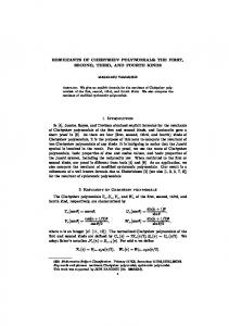
Siemens SP75 G = 865 W/m2 T = (39.5 + 273) K
4
2 1.5 1
0.5
0
5
10
15
Experimental data Five-parameter model data
20 25 V (V)
30
35
40
Proposed model data Seven-parameter model data
Figure 2: 𝐼-𝑉 characteristic for SP75.
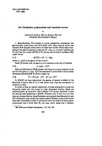
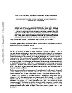
and experimental data. The 𝐼-𝑉 characteristic curves of SP-75 module, MSX-64 module, and APX-90 module at different temperature and irradiance conditions are shown in Figures 2–4, Figures 5–7, and Figures 8–10, respectively. The corresponding absolute errors of 𝐼-𝑉 characteristic curves for these three modules are shown in Figures 11–19. AEs of the six-parameter model in this paper is very close to the sevenparameter model in [13] at every point. For higher irradiance, the absolute errors of the six-parameter model in this paper are less than that of the five-parameter model in [14] within
6
Mathematical Problems in Engineering Table 3: RMSEs of different models for SP75, MSX-64, and APX-90 module.
Module
RMSE Seven-parameter model in [13] 0.056315982 0.125862026 0.147627147
Five-parameter model in [14] 0.06293749 0.130276895 0.154802955
SP75 MSX-64 APX-90
Siemens SP75 G = 520 W/m2 T = (37.2 + 273) K
2.4
3.5
2
3 2.5
1.6 I (A)
I (A)
1.8
1.4 1.2
2 1.5
1
1
0.8
0.5
0.6 0.4
Sloarex MSX-64 G = 865 W/m2 T = (39.3 + 273) K
4
2.2
Six-parameter model 0.056864662 0.125859806 0.147625261
0
5
10
15
Experimental data Five-parameter model data
20 25 V (V)
30
35
0
40
0
Proposed model data Seven-parameter model data
10
15
Experimental data Five-parameter model data
Figure 3: 𝐼-𝑉 characteristic for SP75.
20 25 V (V)
30
35
40
Proposed model data Seven-parameter model data
Figure 5: 𝐼-𝑉 characteristic for MSX-64.
Siemens SP75 G = 298 W/m2 T = (37.1 + 273) K
1.4
5
Sloarex MSX-64 G = 654 W/m2 T = (43.9 + 273) K
3
1.2
2.5
2
0.8
I (A)
I (A)
1
0.6
1.5
0.4 1
0.2 0
0
5
10
15
Experimental data Five-parameter model data
20 25 V (V)
30
35
40
Proposed model data Seven-parameter model data
0.5
0
5
10
15
Experimental data Five-parameter model data
20 25 V (V)
30
35
40
Proposed model data Seven-parameter model data
Figure 4: 𝐼-𝑉 characteristic for SP75.
Figure 6: 𝐼-𝑉 characteristic for MSX-64.
the range of maximum-power point to open-circuit voltage point, shown in Figures 11-12, 14-15, and 17-18. For lower irradiance, AEs of the six-parameter model in this paper and the five-parameter model in [14] are almost the same. In addition, We use the maximum absolute error and RMSE to further analyze the effectiveness of the six-parameter model
in this paper. RMSE shows overall error. We select 97 data sets for SP-75 module, 101 data sets for MSX-64 module and 108 data sets for APX-90 module to compute RMSEs, see Table 3. From Table 3, we can find that that RMSEs of the sixparameter model in this paper are almost the same as that of the seven-parameter model in [13] and are far less than that
Mathematical Problems in Engineering
7
Sloarex MSX-64 G = 298 W/m2 T = (37.4 + 273) K
1.4 1.2
2.5 2
0.8
I (A)
I (A)
1
0.6
1.5 1
0.4
0.5
0.2 0
Anstropower APX-90 G = 520 W/m2 T = (37.7 + 273) K
3
0
10
5
15
20 25 V (V)
Experimental data Five-parameter model data
30
35
0
40
0
Anstropower APX-90 G = 865 W/m2 T = (39.9 + 273) K
20
25
30
Proposed model data Seven-parameter model data
Anstropower APX- 90 G = 298 W/m2 T = (36.9 + 273) K
1.6 1.4
4
1.2
3.5
1
3
I (A)
I (A)
15 V (V)
Figure 9: 𝐼-𝑉 characteristic for APX-90.
4.5
2.5
0.8 0.6
2 1.5
0.4
1
0.2
0.5
10
Experimental data Five-parameter model data
Proposed model data Seven-parameter model data
Figure 7: 𝐼-𝑉 characteristic for MSX-64.
5
5
0
5
10
15 V (V)
Experimental data Five-parameter model data
20
25
30
Proposed model data Seven-parameter model data
0
0
5
10
15 V (V)
Experimental data Five-parameter model data
20
25
30
Proposed model data Seven-parameter model data
Figure 8: 𝐼-𝑉 characteristic for APX-90.
Figure 10: 𝐼-𝑉 characteristic for APX-90.
of the five-parameter model in [14]. Therefore, in estimating of 𝐼-𝑉 characteristic, the six-parameter model in this paper is obviously superior to the five-parameter model in [14], but slightly less than seven-parameter model in [13]. 𝐼-𝑉 characteristic of PV modules are widely used to estimate the maximum power point. Next, we take the data of SM-55 module and US-21 module given in [32] as experimental data to validate the accuracy of the new sixparameter model in estimating the maximum power point. Tables 4 and 5 show 𝑃mp and 𝑉mp for the two PV modules at the temperature of 50∘ C and the irradiance of 1000 W/m2 to 100 W/m2 . For SM-55 module and US-21 module, the relative errors of the six-parameter model in this paper are almost the
same as that of the seven-parameter model in [13]. For SM-55 module, the relative errors of the six-parameter model in this paper are far less than that of five-parameter model in [14] except for irradiance of 1000 W/m2 and 100 W/m2 . For US21 module, the relative errors of the six-parameter model in this paper are far less than that of five-parameter model in [14] except for irradiance of 1000 W/m2 . This shows that the sixparameter model in this paper can give a better estimation of maximum power point at lower irradiance for tripe-junction amorphous silicon module. Therefore, the six-parameter model in this paper, used to estimate 𝐼-𝑉 characteristic and the maximum power point, is obviously superior to the five-parameter model in
100
200
300
400
500
600
700
800
900
1000
𝐺 (W/m2 )
Experimental data 𝑉mp = 15.175 𝑃mp = 47.706 𝑉mp = 15.162 𝑃mp = 42.984 𝑉mp = 15.140 𝑃mp = 38.228 𝑉mp = 15.105 𝑃mp = 33.440 𝑉mp = 15.053 𝑃mp = 28.621 𝑉mp = 14.975 𝑃mp = 23.774 𝑉mp = 14.854 𝑃mp = 18.903 𝑉mp = 14.657 𝑃mp = 14.017 𝑉mp = 14.301 𝑃mp = 9.136 𝑉mp = 13.482 𝑃mp = 4.315
Five-parameter model 𝑉mp = 15.20995 𝑃mp = 48.04719 𝑉mp = 15.24041 𝑃mp = 43.37989 𝑉mp = 15.25940 𝑃mp = 38.65117 𝑉mp = 15.26368 𝑃mp = 33.86514 𝑉mp = 15.24850 𝑃mp = 29.02721 𝑉mp = 15.20650 𝑃mp = 24.14476 𝑉mp = 15.12542 𝑃mp = 19.22832 𝑉mp = 14.98228 𝑃mp = 14.29398 𝑉mp = 14.72561 𝑃mp = 9.36934 𝑉mp = 14.19163 𝑃mp = 4.51282
Seven-parameter model 𝑉mp = 15.06347 𝑃mp = 47.56305 𝑉mp = 15.10802 𝑃mp = 42.99262 𝑉mp = 15.14129 𝑃mp = 38.35024 𝑉mp = 15.16002 𝑃mp = 33.63989 𝑉mp = 15.15945 𝑃mp = 28.86691 𝑉mp = 15.13224 𝑃mp = 24.03857 𝑉mp = 15.06608 𝑃mp = 19.16532 𝑉mp = 14.93800 𝑃mp = 14.26321 𝑉mp = 14.69652 𝑃mp = 9.35976 𝑉mp = 14.17782 𝑃mp = 4.51341
Six-parameter model 𝑉mp = 15.06359 𝑃mp = 47.56339 𝑉mp = 15.10812 𝑃mp = 42.99290 𝑉mp = 15.14138 𝑃mp = 38.35045 𝑉mp = 15.16010 𝑃mp = 33.64005 𝑉mp = 15.15952 𝑃mp = 28.86702 𝑉mp = 15.13228 𝑃mp = 24.03863 𝑉mp = 15.06610 𝑃mp = 19.16534 𝑉mp = 14.93799 𝑃mp = 14.26319 𝑉mp = 14.69648 𝑃mp = 9.35973 𝑉mp = 14.17771 𝑃mp = 4.51337
RE(5-para)% 0.230 at 𝑉mp 0.715 at 𝑃mp 0.517 at 𝑉mp 0.921 at 𝑃mp 0.789 at 𝑉mp 1.107 at 𝑃mp 1.051 at 𝑉mp 1.271 at 𝑃mp 1.299 at 𝑉mp 1.419 at 𝑃mp 1.546 at 𝑉mp 1.560 at 𝑃mp 1.827 at 𝑉mp 1.721 at 𝑃mp 2.219 at 𝑉mp 1.976 at 𝑃mp 2.969 at 𝑉mp 2.554 at 𝑃mp 5.264 at 𝑉mp 4.585 at 𝑃mp
Table 4: Voltage, power, and RE at maximum power point of different models for SM-55 at 𝑇 = 50∘ C. RE(7-para)% 0.735 at 𝑉mp 0.300 at 𝑃mp 0.356 at 𝑉mp 0.020 at 𝑃mp 0.009 at 𝑉mp 0.320 at 𝑃mp 0.364 at 𝑉mp 0.598 at 𝑃mp 0.707 at 𝑉mp 0.859 at 𝑃mp 1.050 at 𝑉mp 1.113 at 𝑃mp 1.428 at 𝑉mp 1.388 at 𝑃mp 1.917 at 𝑉mp 1.757 at 𝑃mp 2.766 at 𝑉mp 2.449 at 𝑃mp 5.161 at 𝑉mp 4.598 at 𝑃mp
RE(6-para)% 0.734 at 𝑉mp 0.299 at 𝑃mp 0.355 at 𝑉mp 0.021 at 𝑃mp 0.009 at 𝑉mp 0.320 at 𝑃mp 0.365 at 𝑉mp 0.598 at 𝑃mp 0.708 at 𝑉mp 0.860 at 𝑃mp 1.050 at 𝑉mp 1.113 at 𝑃mp 1.428 at 𝑉mp 1.388 at 𝑃mp 1.917 at 𝑉mp 1.756 at 𝑃mp 2.765 at 𝑉mp 2.449 at 𝑃mp 5.160 at 𝑉mp 4.597 at 𝑃mp
8 Mathematical Problems in Engineering
100
200
300
400
500
600
700
800
900
1000
𝐺 (W/m2 )
Experimental data 𝑉mp = 15.2 𝑃mp = 19.883 𝑉mp = 15.335 𝑃mp = 18.227 𝑉mp = 15.477 𝑃mp = 16.507 𝑉mp = 15.626 𝑃mp = 14.720 𝑉mp = 15.782 𝑃mp = 12.862 𝑉mp = 15.945 𝑃mp = 10.930 𝑉mp = 16.114 𝑃mp = 8.917 𝑉mp = 16.279 𝑃mp = 6.818 𝑉mp = 16.414 𝑃mp = 4.624 𝑉mp = 16.377 𝑃mp = 2.327
Five-parameter model 𝑉mp = 14.01544 𝑃mp = 18.29121 𝑉mp = 14.33650 𝑃mp = 16.99216 𝑉mp = 14.66351 𝑃mp = 15.57550 𝑉mp = 14.99208 𝑃mp = 14.03842 𝑉mp = 15.31685 𝑃mp = 12.37893 𝑉mp = 15.63061 𝑃mp = 10.59594 𝑉mp = 15.9248 𝑃mp = 8.68954 𝑉mp = 16.17323 𝑃mp = 6.66162 𝑉mp = 16.34112 𝑃mp = 4.51744 𝑉mp = 16.29485 𝑃mp = 2.27106
Seven-parameter model 𝑉mp = 14.84689 𝑃mp = 19.70321 𝑉mp = 15.10970 𝑃mp = 18.15277 𝑉mp = 15.37056 𝑃mp = 16.50499 𝑉mp = 15.62622 𝑃mp = 14.75907 𝑉mp = 15.87229 𝑃mp = 12.91469 𝑉mp = 16.10244 𝑃mp = 10.97225 𝑉mp = 16.30647 𝑃mp = 8.93308 𝑉mp = 16.46573 𝑃mp = 6.80017 𝑉mp = 16.53891 𝑃mp = 4.57978 𝑉mp = 16.39503 𝑃mp = 2.28688
Six-parameter model 𝑉mp = 14.84671 𝑃mp = 19.70291 𝑉mp = 15.10955 𝑃mp = 18.15254 𝑉mp = 15.37044 𝑃mp = 16.50483 𝑉mp = 15.62613 𝑃mp = 14.75896 𝑉mp = 15.87224 𝑃mp = 12.91463 𝑉mp = 16.10243 𝑃mp = 10.97222 𝑉mp = 16.30651 𝑃mp = 8.93309 𝑉mp = 16.46582 𝑃mp = 6.80020 𝑉mp = 16.53908 𝑃mp = 4.57981 𝑉mp = 16.39531 𝑃mp = 2.28691
RE(5-para)% 7.793 at 𝑉mp 8.006 at 𝑃mp 6.511 at 𝑉mp 6.775 at 𝑃mp 5.256 at 𝑉mp 5.643 at 𝑃mp 4.057 at 𝑉mp 4.630 at 𝑃mp 2.947 at 𝑉mp 3.756 at 𝑃mp 1.972 at 𝑉mp 3.056 at 𝑃mp 1.189 at 𝑉mp 2.551 at 𝑃mp 0.650 at 𝑉mp 2.294 at 𝑃mp 0.444 at 𝑉mp 2.305 at 𝑃mp 0.502 at 𝑉mp 2.404 at 𝑃mp
Table 5: Voltage, power, and RE at maximum power point of different models for US-21 at 𝑇 = 50∘ C. RE(7-para)% 2.323 at 𝑉mp 0.904 at 𝑃mp 1.469 at 𝑉mp 0.407 at 𝑃mp 0.688 at 𝑉mp 0.012 at 𝑃mp 0.001 at 𝑉mp 0.265 at 𝑃mp 0.572 at 𝑉mp 0.410 at 𝑃mp 0.987 at 𝑉mp 0.387 at 𝑃mp 1.194 at 𝑉mp 0.180 at 𝑃mp 1.147 at 𝑉mp 0.262 at 𝑃mp 0.761 at 𝑉mp 0.956 at 𝑃mp 0.110 at 𝑉mp 1.724 at 𝑃mp
RE(6-para)% 2.324 at 𝑉mp 0.906 at 𝑃mp 1.470 at 𝑉mp 0.409 at 𝑃mp 0.689 at 𝑉mp 0.013 at 𝑃mp 0.001 at 𝑉mp 0.265 at 𝑃mp 0.572 at 𝑉mp 0.409 at 𝑃mp 0.987 at 𝑉mp 0.386 at 𝑃mp 1.195 at 𝑉mp 0.180 at 𝑃mp 1.148 at 𝑉mp 0.261 at 𝑃mp 0.762 at 𝑉mp 0.956 at 𝑃mp 0.112 at 𝑉mp 1.723 at 𝑃mp
Mathematical Problems in Engineering 9
10
Mathematical Problems in Engineering Siemens SP75 G = 865 W/m2 T = (39.5 + 273) K
0.2 0.18
0.16
0.16
0.14 Absolute error (A)
Absolute error (A)
0.14 0.12 0.1 0.08 0.06
0.12 0.1 0.08 0.06 0.04
0.04
0.02
0.02 0
Siemens SP75 G = 298 W/m2 T = (37.1 + 273) K
0.18
0
5
10
15
20
25
30
35
0
40
0
5
10
15
V (V) Five-parameter model Seven-parameter model
Five-parameter model Seven-parameter model
Proposed model
Siemens SP75 G = 520 W/m2 T = (37.2 + 273) K
35
40
Proposed model
0.2 Absolute error (A)
Absolute error (A)
30
Solarex MSX-64 G = 865 W/m2 T = (39.3 + 273) K
0.25
0.2
0.15
0.1
0.15
0.1
0.05
0.05
0
25
Figure 13: Absolute error for SP75.
Figure 11: Absolute error for SP75.
0.25
20 V (V)
0
5
10
15
20 V (V)
Five-parameter model Seven-parameter model
25
30
35
40
Proposed model
Figure 12: Absolute error for SP75.
[14] under most weather conditions, and is close to sevenparameter model in [13]. In fact, the six-parameter model in this paper makes a good compromise between the fiveparameter model in [14] and the seven-parameter model in [13] at accuracy and computational complexity. Therefore, the six-parameter model is an 𝐼-𝑉 model with moderate computational complexity and high precision.
5. Conclusions We propose a new six-parameter model for solar cells in this paper. At calculation accuracy, the six-parameter model is better than the five-parameter model. The prediction of
0
0
5
10
15
20 V (V)
Five-parameter model Seven-parameter model
25
30
35
40
Proposed model
Figure 14: Absolute error for MSX-64.
𝐼-𝑉 characteristic of six-parameter model is very close to the seven-parameter model, but less than seven-parameter model. However, at the computational complexity, the sixparameter model is superior to the seven-parameter model. Experiment results show that the new six-parameter model can provide a good prediction for silicon solar cells with different technology types, that is, monocrystalline silicon, polycrystalline silicon, thin film silicon, and tripe-junction amorphous silicon. That is to say, the model in this paper is more universal. It is worth mentioning that the relationship between the series resistance and temperature is described by using Chebyshev polynomials in this paper. Therefore, the six-parameter model proposed in this paper is an 𝐼-𝑉 model with moderate computational complexity and high precision.
Mathematical Problems in Engineering
11
Solarex MSX-64 G = 654 W/m2 T = (43.9 + 273) K
0.4 0.35
0.2 Absolute error (A)
0.3 Absolute error (A)
Anstropower APX-90 G = 865 W/m2 T = (39.9 + 273) K
0.25
0.25 0.2 0.15 0.1
0.15
0.1
0.05
0.05 0
0
5
10
15
20 V (V)
Five-parameter model Seven-parameter model
25
30
35
0
40
0
Solarex MSX-64 G = 298 W/m2 T = (37.4 + 273) K
25
30
Proposed model
0.6 0.5
0.2
Absolute error (A)
Absolute error (A)
20
Anstropower APX-90 G = 520 W/m2 T = (37.7 + 273) K
0.7
0.25
0.15 0.1 0.05
0.4 0.3 0.2 0.1
0
5
10
15
20 V (V)
Five-parameter model Seven-parameter model
25
30
35
Proposed model
Figure 16: Absolute error for MSX-64.
Nomenclature 𝑎:
15 V (V)
Figure 17: Absolute error for APX-90.
0.3
0
10
Five-parameter model Seven-parameter model
Proposed model
Figure 15: Absolute error for MSX-64.
0.35
5
Ideality factor parameter which is defined as 𝑎 ≡ 𝑁𝑠 𝑛𝐼 𝑉𝑡 𝑎ref : Ideality factor parameter at SRC 𝐸𝑔 : Energy bandgap (eV) 𝐸𝑔,ref : Energy bandgap at SRC (eV) 𝐺: Solar irradiance (W/m2 ) 𝐺ref : Solar irradiance at SRC (W/m2 ) 𝐼: Current (A) Light-generated current (A) 𝐼𝐿 : 𝐼𝐿,ref : Light-generated current at SRC (A) 𝐼mp : The current at maximum power point (A)
40
0
0
5
10
15 V (V)
Five-parameter model Seven-parameter model
20
25
Proposed model
Figure 18: Absolute error for APX-90.
𝐼mp,ref : The current at maximum power point at SRC (A) Diode reverse saturation current (A) 𝐼𝑜 : 𝐼𝑜,ref : Diode reverse saturation current at SRC (A) Short-circuit current (A) 𝐼sc : 𝐼sc,ref : Short-circuit current at SRC (A) 𝑘: Boltzmann’s constant (1.38066𝐸 − 23 J/K) Diode ideality factor 𝑛𝐼 : Number of solar cells in series in one module 𝑁𝑠 : 𝑃mp : Power at maximum power point (W) 𝑃mp,ref : Power at maximum power point at SRC (W) 𝑞: Electron charge (1.60218𝐸 − 19 C)
30
12
Mathematical Problems in Engineering Anstropower APX-90 G = 298 W/m2 T = (36.9 + 273) K
0.7
the Nature Science Foundation of Liaoning Province under Grants 201102005 and 201402014, the First Batch of Science and Technology Projects of Liaoning Province under Grant 2011402001, and Liaoning BaiQianWan Talents Program under Grant 2012921061.
0.6
Absolute error (A)
0.5 0.4
References
0.3
[1] H. G. Zhang, T. D. Ma, and G.-B. Huang, “Robust global exponential synchronization of uncertain chaotic delayed neural networks via dual-stage impulsive control,” IEEE Transactions on Systems, Man, and Cybernetics. Part B: Cybernetics, vol. 40, no. 3, pp. 831–844, 2010. [2] H. G. Zhang, B. Jiang, and W. Yu, “Data-driven fault supervisory control theory and applications,” Mathematical Problems in Engineering, vol. 2013, Article ID 387341, 2 pages, 2013. [3] H. G. Zhang, C. B. Qin, B. Jiang, and Y. H. Luo, “Online adaptive policy learning algorithm for 𝐻∞ state feedback control of unknown affine nonliear discretetime systems,” IEEE Transactions on Cybernetics, vol. 44, no. 12, pp. 2706–2718, 2014. [4] H. G. Zhang, Q. Wang, E. H. Chu, X. Liu, and L. Hou, “Analysis and implementation of a passive lossless soft-switching snubber for PWM inverters,” IEEE Transactions on Power Electronics, vol. 26, no. 2, pp. 411–426, 2011. [5] Q. Wang, H.-G. Zhang, E.-H. Chu, X.-C. Liu, and L.-M. Hou, “A novel three-phase passive soft-switching inverter,” Proceedings of the Chinese Society of Electrical Engineering, vol. 29, no. 18, pp. 33–40, 2009. [6] H.-G. Zhang, Q. Wang, E.-H. Chu, L.-M. Hou, and C. Chen, “A novel resonant DC link soft-switching inverter,” Proceedings of the Chinese Society of Electrical Engineering, vol. 30, no. 3, pp. 21–27, 2010. [7] S.-X. Lun, C.-J. Du, T.-T. Guo, S. Wang, J.-S. Sang, and J.-P. Li, “A new explicit I-V model of a solar cell based on taylor’s series expansion,” Solar Energy, vol. 94, pp. 221–232, 2013. [8] K. M. El-Naggar, M. R. AlRashidi, M. F. AlHajri, and A. K. Al-Othman, “Simulated Annealing algorithm for photovoltaic parameters identification,” Solar Energy, vol. 86, no. 1, pp. 266– 274, 2012. [9] S. X. Lun, C. J. Du, G. H. Yang et al., “An explicit approximate I–V characteristic model of a solar cell based on pad´e approximants,” Solar Energy, vol. 92, pp. 147–159, 2013. [10] A. Askarzadeh and A. Rezazadeh, “Parameter identification for solar cell models using harmony search-based algorithms,” Solar Energy, vol. 86, no. 11, pp. 3241–3249, 2012. [11] A. N. Celik and N. Acikgoz, “Modelling and experimental verification of the operating current of mono-crystalline photovoltaic modules using four- and five-parameter models,” Applied Energy, vol. 84, no. 1, pp. 1–15, 2007. [12] W. de Soto, S. A. Klein, and W. A. Beckman, “Improvement and validation of a model for photovoltaic array performance,” Solar Energy, vol. 80, no. 1, pp. 78–88, 2006. [13] T. Boyd, Evaluation and validation of equivalent circuit photovoltaic solar cell performance models [M.S. thesis], Mechanical Engineering, Univerisity of Wisconsin-Madison, 2010. [14] W. De Soto, Improved approximate analytical solution for generalized diode equation [M.S. thesis], Mechanical Engineering, University of Wisconsin-Madison, 2004. [15] J. M. Ma, T. O. Ting, K. L. Man, N. Zhang, S.-U. Guan, and P. W. Wong, “Parameter estimation of photovoltaic models
0.2 0.1 0
0
5
10
15
20
25
30
V (V) Five-parameter model Seven-parameter model
Proposed model
Figure 19: Absolute error for APX-90.
𝛿: 𝑅𝑠 : 𝑅𝑠,ref : 𝑅sh : 𝑅sh,ref : 𝑇: 𝑇ref : 𝑉: 𝑉mp : 𝑉mp,ref :
Temperature coefficient for series resistance Series resistance (Ω) Series resistance at SRC (Ω) Shunt resistance (Ω) Shunt resistance at SRC (Ω) Cell temperature (K) Cell temperature at SRC (K) Voltage (V) The voltage at maximum power point (V) The voltage at maximum power point at SRC (V) Open-circuit voltage (V) 𝑉oc : 𝑉oc,ref : Open-circuit voltage at SRC (V) Thermal voltage (V) 𝑉𝑡 : 𝛼𝐼mp : Temperature coefficient for maximum power current (A/K) Temperature coefficient for short-circuit 𝛼𝐼sc : current (A/K) 𝛽𝑉mp : Temperature coefficient for maximum power voltage (V/K) 𝛽𝑉oc : Temperature coefficient for open-circuit voltage (V/K) 𝛾𝑃mp : Temperature coefficient for maximum power (1/K) Temperature changing factor. Δ 𝑇:
Conflict of Interests The authors declare that there is no conflict of interests regarding the publication of this paper.
Acknowledgments This work was supported by the Program for New Century Excellent Talents in University under Grant NCET-11-1005,
Mathematical Problems in Engineering
[16]
[17]
[18]
[19]
[20]
[21]
[22]
[23]
[24]
[25]
[26]
[27]
[28]
[29]
[30] [31] [32]
via cuckoo search,” Journal of Applied Mathematics, vol. 2013, Article ID 362619, 8 pages, 2013. J. Appelbaum and A. Peled, “Parameters extraction of solar cells—a comparative examination of three methods,” Solar Energy Materials & Solar Cells, vol. 122, pp. 164–173, 2014. C. Wen, C. Fu, J. L. Tang, D. X. Liu, S. F. Hu, and Z. G. Xing, “The influence of environment temperatures on single crystalline and polycrystalline silicon solar cell performance,” Science China: Physics, Mechanics and Astronomy, vol. 55, no. 2, pp. 235–241, 2012. M. Lal and S. N. Singh, “A new method of determination of series and shunt resistances of silicon solar cells,” Solar Energy Materials and Solar Cells, vol. 91, no. 2-3, pp. 137–142, 2007. M. A. de Blas, J. L. Torres, E. Prieto, and A. Garc´ıa, “Selecting a suitable model for characterizing photovoltaic devices,” Renewable Energy, vol. 25, no. 3, pp. 371–380, 2002. D. T. Cotfas, P. A. Cotfas, and S. Kaplanis, “Methods to determine the dc parameters of solar cells: a critical review,” Renewable and Sustainable Energy Reviews, vol. 28, pp. 588–596, 2013. P. Singh, S. N. Singh, M. Lal, and M. Husain, “Temperature dependence of I-V characteristics and performance parameters of silicon solar cell,” Solar Energy Materials and Solar Cells, vol. 92, no. 12, pp. 1611–1616, 2008. M. Sheraz Khalid and M. Abido, “A novel and accurate photovoltaic simulator based on seven-parameter model,” Electric Power Systems Research, vol. 116, pp. 243–251, 2014. A. Tataro˘glu and S¸. Altindal, “The analysis of the series resistance and interface states of MIS Schottky diodes at high temperatures using I−V characteristics,” Journal of Alloys and Compounds, vol. 484, no. 1-2, pp. 405–409, 2009. A. K. Das, “Analytical expression of the physical parameters of an illuminated solar cell using explicit J-V model,” Renewable Energy, vol. 52, pp. 95–98, 2013. S. Daliento and L. Lancellotti, “3D Analysis of the performances degradation caused by series resistance in concentrator solar cells,” Solar Energy, vol. 84, no. 1, pp. 44–50, 2010. Y. Li, W. X. Huang, H. Huang et al., “Evaluation of methods to extract parameters from current-voltage characteristics of solar cells,” Solar Energy, vol. 90, pp. 51–57, 2013. J. L. Ding, X. F. Cheng, and T. R. Fu, “Analysis of series resistance and P-T characteristics of the solar cell,” Vacuum, vol. 77, no. 2, pp. 163–167, 2005. E. Cuce, P. M. Cuce, and T. Bali, “An experimental analysis of illumination intensity and temperature dependency of photovoltaic cell parameters,” Applied Energy, vol. 111, pp. 374–382, 2013. A. Redinger, M. Mousel, M. H. Wolter, N. Valle, and S. Siebentritt, “Influence of S/Se ratio on series resistance and on dominant recombination pathway in Cu2 ZnSn(SSe)4 thin film solar cells,” Thin Solid Films, vol. 535, no. 1, pp. 291–295, 2013. Y. Jin and Y. Chen, Numerical Method, China Machine Press, 2004. R. Burden and J. Faires, Numerical Analysis, Thomson Learning Press, 2003. E. Karatepe and T. Hiyama, “Polar coordinated fuzzy controller based real-time maximum-power point control of photovoltaic system,” Renewable Energy, vol. 34, no. 12, pp. 2597–2606, 2009.
13
Advances in
Operations Research Hindawi Publishing Corporation http://www.hindawi.com
Volume 2014
Advances in
Decision Sciences Hindawi Publishing Corporation http://www.hindawi.com
Volume 2014
Journal of
Applied Mathematics
Algebra
Hindawi Publishing Corporation http://www.hindawi.com
Hindawi Publishing Corporation http://www.hindawi.com
Volume 2014
Journal of
Probability and Statistics Volume 2014
The Scientific World Journal Hindawi Publishing Corporation http://www.hindawi.com
Hindawi Publishing Corporation http://www.hindawi.com
Volume 2014
International Journal of
Differential Equations Hindawi Publishing Corporation http://www.hindawi.com
Volume 2014
Volume 2014
Submit your manuscripts at http://www.hindawi.com International Journal of
Advances in
Combinatorics Hindawi Publishing Corporation http://www.hindawi.com
Mathematical Physics Hindawi Publishing Corporation http://www.hindawi.com
Volume 2014
Journal of
Complex Analysis Hindawi Publishing Corporation http://www.hindawi.com
Volume 2014
International Journal of Mathematics and Mathematical Sciences
Mathematical Problems in Engineering
Journal of
Mathematics Hindawi Publishing Corporation http://www.hindawi.com
Volume 2014
Hindawi Publishing Corporation http://www.hindawi.com
Volume 2014
Volume 2014
Hindawi Publishing Corporation http://www.hindawi.com
Volume 2014
Discrete Mathematics
Journal of
Volume 2014
Hindawi Publishing Corporation http://www.hindawi.com
Discrete Dynamics in Nature and Society
Journal of
Function Spaces Hindawi Publishing Corporation http://www.hindawi.com
Abstract and Applied Analysis
Volume 2014
Hindawi Publishing Corporation http://www.hindawi.com
Volume 2014
Hindawi Publishing Corporation http://www.hindawi.com
Volume 2014
International Journal of
Journal of
Stochastic Analysis
Optimization
Hindawi Publishing Corporation http://www.hindawi.com
Hindawi Publishing Corporation http://www.hindawi.com
Volume 2014
Volume 2014