A New Solution Path Algorithm in Support Vector Regression

1

A New Solution Path Algorithm in Support Vector Regression

Gang Wang, Dit-Yan Yeung, Frederick H. Lochovsky

The authors are with the Hong Kong University of Science and Technology. June 11, 2008

DRAFT

2

Abstract Regularization path algorithms were proposed as a novel approach to the model selection problem by exploring the path of possibly all solutions with respect to some regularization hyperparameter in an efficient way. This approach was later extended to a support vector regression (SVR) model called -SVR. However, the method requires that the error parameter  be set a priori. This is only possible if the desired accuracy of the approximation can be specified in advance. In this paper, we analyze the solution space for -SVR and propose a new solution path algorithm, called -path algorithm, which traces the solution path with respect to the hyperparameter  rather than λ. Although both two solution path algorithms possess the desirable piecewise linearity property, our -path algorithm overcomes some limitations of the original λ-path algorithm and has more advantages. It is thus more appealing for practical use.

Index Terms Solution Path, Support Vector Regression, Model Selection

I. I NTRODUCTION In a typical regression problem, we are given a training set of independent and identically distributed (i.i.d.) examples in the form of n ordered pairs, {(xi , yi )}ni=1 ⊂ Rd × R, where xi and yi denote the input and output, respectively, of the ith training example. Linear regression is the simplest method to solve the regression problem where the regression function is a linear function of the input. As a nonlinear extension, support vector regression (SVR) is a kernel method which extends linear regression to nonlinear regression by exploiting the kernel trick [1], [2]. Essentially, each input xi ∈ Rd is mapped implicitly via a nonlinear feature map φ(·) to some kernel-induced feature space F where linear regression is performed. Specifically, SVR learns the following regression function by estimating w ∈ F and w0 ∈ R from the training data: f (x) = hw, φ(x)i + w0 ,

(1)

where h·, ·i denotes the inner product in F. The problem is solved by minimizing some empirical risk measure that is regularized appropriately to control the model capacity. One commonly used SVR model is called -SVR. In the -SVR model, the -insensitive loss function |y − f (x)| = max{0, |y − f (x)| − } is used to define an empirical risk functional June 11, 2008

DRAFT

3

ξ

(a) Fig. 1.

(b)

(c)

(d)

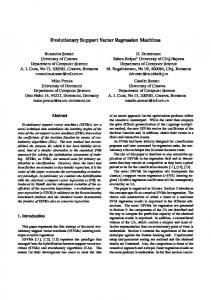
Linear SVR results for four different combinations of values for λ and . (a) proper values of λ and  are specified;

(b) λ = ∞; (c)  > (ymax − ymin )/2; (d)  < (ymax − ymin )/2, but all the data points are inside the -tube.

which exhibits the same sparseness property as that for support vector classifiers (SVC) using the hinge loss function via the so-called support vectors (SV). If a data point x lies inside the insensitive zone called the -tube, i.e., |y − f (x)| ≤ , then it will not incur any loss. However, the error parameter  ≥ 0 has to be specified a priori by the user. The primal optimization problem for -SVR can be stated as follows: n

min

w,ξ (∗)

subject to

X λ kwk2 + (ξi + ξi∗ ) 2 i=1

(2)

yi − (hw, φ(xi )i + w0 ) ≤  + ξi

(3)

(hw, φ(xi )i + w0 ) − yi ≤  + ξi∗

(4)

(∗)

ξi Here and below, i = 1, . . . , n and

(∗)

≥ 0.

(5)

denote both the variables with and without asterisks. The

regularization hyperparameter λ > 0 plays a role in capacity control by maintaining a proper balance between empirical loss and model complexity. Like , λ also has to be chosen in advance by the user. The two hyperparameters λ and  play different roles in -SVR. Figure 1 shows four different combinations of the hyperparameter values. In practice, users often use some default values for λ and  even though they are by no means optimal choices. A better approach is to specify some candidate hyperparameter values and then apply cross validation to select the best choices among the candidates. However, extensive exploration for the optimal hyperparameter values is seldom pursued since this requires training the model many times under different hyperparameter settings. To overcome the difficulty of selecting , [3] proposed the ν-SVR model which automatically adjusts the width of the tube June 11, 2008

DRAFT

4

so that at most a fraction ν of the data points lie outside the tube. Although ν-SVR can help alleviate much of the effort involved in choosing the  value, it is still very time consuming to find an appropriate combination of values for λ and  to fit the data. More recently, a novel approach has emerged to address the model selection problem by exploring the entire regularization path1 for solutions without having to re-train the model multiple times [4]–[8]. Research efforts in this direction have resulted in several regularization path algorithms. For SVR, [9] devised an algorithm that computes the entire solution path with respect to λ for some fixed  value. The algorithm starts from λ = ∞, with the initial solution obtained by solving a linear programming problem. As λ decreases, the algorithm computes the solution for every value of λ. However, we observe that sometimes the regularization path cannot be traced successfully during the execution of the algorithm. When there exists only one or even no point at the boundaries, the tube has to move and rotate until two valid points enter the tube. There exist many possible combinations for two points to enter the elbows simultaneously. Hence, the algorithm needs to enumerate all the combinations and then pick a valid one from them. However, since the search strategy to enumerate all possible combinations is not systematic, this difficulty will pose a problem to the algorithm. As a consequence, it is not easy to realize the λ-path algorithm in practice. In this paper, we also address the solution path problem for -SVM. Our main contributions can be summarized by these two key findings: •

We establish that the dual variables of the dual optimization problem corresponding to (2) are piecewise linear with respect to the two-dimensional hyperparameter vector (λ, );

•

We propose an efficient solution path algorithm, called -path algorithm, that traces the solution path with respect to  for the optimization problem in (2) when λ is fixed.

Our -path algorithm possesses competitive advantages over the λ-path algorithm proposed by [9]. Not only can the -path algorithm always proceed without difficulty, but it also has a very simple initialization step and is efficient in finding a good regression function that can generalize well. More specifically, the -path algorithm initializes the tube width to infinity, implying that it starts with no support vectors. The algorithm then reduces the tube width so that the number of support vectors increases gradually as the algorithm proceeds. As a result, a good regression 1

For notation simplicity, we refer to the regularization path as λ-path.

June 11, 2008

DRAFT

5

function with the desirable sparseness property can be obtained only after a small number of iterations in decreasing . The rest of this paper is organized as follows. Section II briefly reviews some existing solution path algorithms and Section III reviews the -SVR formulation and introduces some basic terminology used later in the paper. In Section IV, we present a new approach for devising solution path algorithms and investigate the use of this approach for both the λ-path and the -path. Some further discussions are given in Section V and experimental results are presented in Section VI. Finally, the last section concludes the paper. II. S OLUTION PATH A LGORITHMS The basic idea underlying solution path algorithms comes from continuation methods [10], which compute the current solution based on an already obtained one. Specifically, we can interpret a solution path algorithm as follows: given a hyperparameter value µ and its corresponding solution fˆµ ,2 a solution path algorithm seeks to update the solution from fˆµ to fˆµ+s in an efficient way as µ changes to µ + s by a small value s. The updating formula is often expressed as fˆµ+s = fˆµ + u(µ, s). If the solution changes nonlinearly with s, gradient descent or the Newton-Raphson method [11] can be used to estimate u(µ, s). On the other hand, if the solution changes linearly with s, u(µ, s) can be expressed as s·v(µ) where v(µ) does not depend on s. This approach makes it possible to trace the (entire) solution path as a function of the hyperparameter without having to train the model multiple times. Cross validation may then be used to estimate the hyperparameter value that gives the lowest generalization error. Since this approach has much lower computational demand without the need for training the model multiple times, we can afford to estimate the generalization errors for a much larger set of hyperparameter values in searching for the optimal choice. Previous works mainly focus on exploring the solution path with respect to the regularization hyperparameter and hence the resulting solution path is also called regularization path. [6] proposed an algorithm called the least angle regression (LARS) algorithm. It can be used to trace the regularization path for linear least square regression As the hyperparameter value µ changes, the solution estimator fˆ will change accordingly. Thus the estimator can be considered as a function of µ. We use fˆµ to indicate the dependence on µ. 2

June 11, 2008

DRAFT

6

regularized with the L1 norm. An important finding is that the path of the solutions is piecewise linear and hence it is efficient to explore the entire path by monitoring the breakpoints between the linear segments only. [7] proposed an algorithm to compute the regularization path for the standard L2 -norm SVC and [5] proposed one for the L1 -norm SVC. They are again based on the property that the paths are piecewise linear with respect to the regularization hyperparameter. [12] showed that boosting approximately follows the regularization path with an appropriate loss and an L1 penalty. More generally, [4] showed that any model with an L1 regularization term and a quadratic, piecewise quadratic, piecewise linear, or linear loss function has a piecewise linear solution path and hence the entire path can be computed efficiently. For general loss functions and regularizers, the regularization paths are typically not (piecewise) linear. The predictor-corrector algorithm [10] is one of the fundamental strategies for implementing numerical continuation methods and can be used for tracing the solution path. [11] proposed another path-following algorithm for approximating nonlinear solution paths. In this paper, we investigate the solution space of -SVR based on a novel view. In particular, we consider two types of optimality conditions, namely, equality conditions and inequality conditions, which play different roles in exploring the solution space: • The equalities establish conditions that must be satisfied throughout the entire solution path •

and thus determine the direction of movement between breakpoints; The inequalities determine which data points are involved in the equality constraints and thus determine the breakpoints.

Based on this approach, it is straightforward to investigate the path-following algorithm for either λ or . An advantage of this approach is that it is very general and can be applied to explore the solution paths for other hyperparameters as well.

June 11, 2008

DRAFT

7

III. SVR P ROBLEM F ORMULATION Applying the method of Lagrange multipliers to the primal optimization problem for -SVR in (2)–(5), we arrive at the following dual optimization problem: max α(∗)

n 1 X − (αi − αi∗ )(αj − αj∗ )K(xi , xj ) 2λ i,j=1

−

n X

(αi +

αi∗ )

n X + (αi − αi∗ )yi

i=1

subject to

(6)

i=1

(∗)

0 ≤ αi ≤ 1 n X (αi − αi∗ ) = 0,

(7) (8)

i=1

where K(xi , xj ) = hφ(xi ), φ(xj )i is the kernel function specified by the user and αi and αi∗ are the Lagrange multipliers for constraints (3) and (4), respectively. We also have

n

1X (αi − αi∗ )φ(xi ). w= λ i=1

(9)

By substituting (9) into (1), the regression function can be rewritten as: f (x) = hw, φ(x)i + w0 n 1X = (αi − αi∗ )K(xi , x) + w0 . λ i=1

(10)

From the Karush-Kuhn-Tucker (KKT) optimality conditions, we can derive the following relationships: yi − f (xi ) >  =⇒ αi = 1, αi∗ = 0

(11)

yi − f (xi ) =  =⇒ αi ∈ [0, 1], αi∗ = 0

(12)

yi − f (xi ) ∈ (−, ) =⇒ αi = 0, αi∗ = 0

(13)

yi − f (xi ) = − =⇒ αi = 0, αi∗ ∈ [0, 1]

(14)

yi − f (xi ) < − =⇒ αi = 0, αi∗ = 1

(15)

As a consequence, f (x) can be expressed as an expansion in terms of only a subset of data points for which either αi or αi∗ is nonzero. These points are referred to as SVs which, like those

June 11, 2008

DRAFT

8

Loss Left elbow(EL) Right elbow(ER)

Left of elbows(L)

Fig. 2.

Center(C)



Right of elbows(R) y − f(x)

The set of all data points is partitioned into five subsets according to the -insensitive loss function.

for SVC, contribute to the sparseness property of f (x) with representational and computational advantages.3 Following the convention in [9], we partition the set of all data points into the following five subsets as illustrated in Figure 2: •

R = {i : yi − f (xi ) > , αi = 1, αi∗ = 0} (Right of the elbows)

•

ER = {i : yi − f (xi ) = , αi ∈ [0, 1], αi∗ = 0} (Right elbow)

•

C = {i : |yi − f (xi )| < , αi = 0, αi∗ = 0} (Center)

•

EL = {i : yi − f (xi ) = −, αi = 0, αi∗ ∈ [0, 1]} (Left elbow)

•

L = {i : yi − f (xi ) < −, αi = 0, αi∗ = 1} (Left of the elbows)

As we change the value of λ or , the tube will move, rotate, shrink, expand or remain unchanged. Some events may occur during this process. An event is said to occur when a point enters or leaves an elbow, causing some point sets to change as a result. We categorize the different events as follows: 1) A point enters an elbow:

3

•

From C to ER with αi = 0

•

From C to EL with αi∗ = 0

•

From R to ER with αi = 1

The notion of sparsity here is somewhat different from that commonly used in statistics in the context of variable selection.

As a kernel method, the sparseness property of f (x) refers to a regression function that is represented as a linear combination of a small number of kernel function terms. June 11, 2008

DRAFT

9

From L to EL with αi∗ = 1 2) A point leaves an elbow: •

•

From ER to R with αi = 1

•

From ER to C with αi = 0

•

From EL to C with αi∗ = 0

•

From EL to L with αi∗ = 1 (∗)

For those points lying inside or outside the tube, i.e., in R ∪ C ∪ L, their αi

values remain fixed

until an event occurs. Hence, it suffices to focus on the points at the elbows, i.e., in ER ∪ EL . IV. SVR S OLUTION PATHS A. Optimality Conditions The SVR dual optimization problem in (6)–(8) is a quadratic programming (QP) problem. When the kernel matrix K = (K(xi , xj )) is positive semi-definite, the problem has a unique optimal solution. For the convenience of subsequent derivation, we define α0 = λw0 and rewrite the regression function in (10) as " n # 1 X f (x) = (αi − αi∗ )K(xi , x) + α0 . λ i=1

(16)

In the dual optimization problem, convex optimization is performed on a feasible set defined by the constraints (7) and (8). However, when the KKT conditions (11)–(15) play a role in defining the optimality conditions, (α(∗) , α0 ) is the optimal solution if and only if it satisfies all these conditions. Thus, (7)–(8) and (11)–(15) comprise the optimality conditions for SVR. The optimality conditions can be distinguished into the equality conditions (8), (12) and (14) and the inequality conditions (7), (11), (13) and (15). The equality conditions (12) and (14), which hold only for the points at the elbows (i.e., in ER ∪ EL ), lead to the following linear system: X

αi K(xi , xj ) −

i∈ER

X

αi∗ K(xi , xj ) + α0

i∈EL

= λ(yj − ) −

X

αi K(xi , xj ) +

i∈R

X

= λ(yk + ) −

(17)

X

αi∗ K(xi , xk ) + α0

i∈EL

X i∈R

June 11, 2008

αi∗ K(xi , xj ), ∀j ∈ ER ,

i∈L

αi K(xi , xk ) −

i∈ER

X

αi K(xi , xk ) +

X

αi∗ K(xi , xk ), ∀k ∈ EL .

(18)

i∈L DRAFT

10

From another equality condition (8), we have X X X X αi − αi + αi∗ . αi∗ = − i∈ER

i∈EL

i∈R

(19)

i∈L

Suppose ER contains p1 indices and EL contains p2 indices. The value p1 + p2 indicates the total number of points at the elbows. The size of the linear system defined by (17)–(19) is thus equal to p = p1 + p2 + 1. The system of p   α0  Ka  αER  −α∗EL

linear equations can be represented in matrix form as     0      (20)  = λyE + λ1a − Kb  αR  .    −α∗L

where the undefined notations are introduced in the Appendix. Suppose we have an SVR solution for certain hyperparameters (λ, ). According to the regression function of this solution, data points are partitioned into five subsets as defined above. As the hyperparameter λ or  changes its value, the solution will change accordingly in order to satisfy equation (20). We consider the period between two consecutive events when αR and α∗L remain unchanged at 0 or 1. During this period, only those points at the elbows (i ∈ ER ∪ EL ) can change their values. From the equality condition (8), we know that if one point at an elbow changes its value, then at least one other elbow point must also modify its value correspondingly. An immediate consequence of this is that there should be at least two points at the elbows, i.e., p1 + p2 ≥ 2.4 When a new hyperparameter value is specified, the corresponding solution can be computed as 







 α0   0      (21)  αER  = λ(Ka )−1 (yE + 1a ) − (Ka )−1 Kb  αR  .     −α∗EL −α∗L    α0    It is easy to see that  αER  is linear in either λ or . If the inverse of Ka does not exist,   α∗EL the update of the solution will no longer be unique. For the sake of illustration, we consider an example where the points {xi } are from a one-dimensional space. When a linear kernel is 4

If p1 + p2 < 2, we face a problem in the initialization setup. The algorithms for the λ-path and the -path use different

methods to handle this case. We will discuss them in Sections IV-B and IV-C, respectively.

June 11, 2008

DRAFT

11

applied and there exist three points at the elbows, the kernel matrix Ka is not of full rank. As a result, the solution path algorithm can have multiple updating possibilities with each one corresponding to choosing any two of the three points to compute a new solution. In this paper, we exclude this case by considering the positive definite kernels only. When the kernels are positive semidefinite, the optimal solution may not be unique. We modify Ka by adding a ridge term to ensure that (Ka )−1 always exists and an approximate path of solutions is obtained. The p linear equations above have been used to derive the updating formula for a new solution. However, the derivation is based on the assumption that no event occurs during the period even though the hyperparameter value has changed. Hence, given a certain hyperparameter value and the solution obtained for that value, the solutions for new hyperparameter values within a local neighborhood in which no event occurs can be computed directly via equation (21). On the other hand, the inequality conditions serve to indicate when the assumption no longer holds. When a new solution along the path violates the inequality conditions, the point sets have to be updated to determine the next breakpoint. Here, we consider the algorithm to trace the λ-path from λl in the decreasing direction. Tracing the λ-path in the increasing direction and tracing the -path are both very similar to this. We simplify equation (21) to 

 α0   αER  −α∗EL

    = λva − vb , 

(22)

where va = (v0a , via (∀i ∈ ER ), vja (∀j ∈ EL ))T = (Ka )−1 (yE + 1a )   0  vb = (v0b , vib (∀i ∈ ER ), vjb (∀j ∈ EL ))T = (Ka )−1 Kb  αR  −α∗L

(23)     

(24)

are independent of λ. The algorithm monitors the occurrence of any of these possible events: •

l The αi or αi∗ value of a point i ∈ ER ∪ ELl reaches 0 or 1. The λi value of the point can be

calculated by λi = (αi + vib )/via (∀i ∈ ER ) or λi = (−αi∗ + vib )/via (∀i ∈ EL ). •

A point i ∈ Rl ∪ C l ∪ Ll hits an elbow, i.e., |yi − f (xi )| = . The λi value of the point can be calculated directly by plugging (22) into (16).

June 11, 2008

DRAFT

12

Since the solution is linear in either λ or , the λi values for the possible events above can be computed exactly. Through monitoring these possible breakpoint values, we can find the next breakpoint, λl+1 = arg maxi {λi < λl }, at which the next event occurs. The algorithm then updates the point sets before decreasing the hyperparameter value further. This updating step is essential, or else the solutions computed for the hyperparameter values beyond the breakpoint without updating the point sets will lead to violation of the inequality conditions. We thus have an algorithm for tracing the SVR solutions along the λ-path or the -path. However, since the λ-path and -path have different properties, we will discuss them separately in the next two subsections. B. λ-Path The λ-path algorithm discussed above is essentially the same as the regularization path algorithm proposed by [9]. However, the algorithm derived based on our approach for computing the next breakpoint via (22) is simpler and easier to understand. The λ-path algorithm explores the correspondence between every λ value and the corresponding solution (α(∗) (λ), w0 (λ)) while  is fixed. The path may start from the solution of an -SVR model for any initial value of λ, (∗)

since the values of αi

fully determine the sets R, ER , C, EL and L. However, this requires

solving a QP problem which is computationally demanding if it is solved directly. The problem becomes simpler if we set λ = ∞ initially. Doing so will make the first term of the objective function (6) vanish, leaving only the last two terms. Thus the QP problem degenerates to a linear programming problem which is easier to solve. Similarly, the first term of (10) vanishes so that the regression function becomes f (x) = w0 , which corresponds to the case shown in (∗)

(∗)0

Figure 1(b). The initial values of αi , denoted as αi

, are either 0 or 1 if all the values of

yi are distinct. The -tube is bounded by the sets R, C and L. The tube can move around by changing λ and w0 , while no point is allowed to pass through any elbow. Hence the following constraints are satisfied: 1X 0 (αi − αi∗0 )K(xi , xj ) − w0 >  for j ∈ R yj − λ i 1X 0 (αi − αi∗0 )K(xi , xj ) − w0 <  for j ∈ C y j − λ i 1X 0 yj − (αi − αi∗0 )K(xi , xj ) − w0 < − for j ∈ L λ i June 11, 2008

(25) (26) (27)

DRAFT

13

invalid

valid

Fig. 3. The tube rotates in a clockwise direction as λ decreases. The one on the left is the initial case. Shown on the right are three possible rotation results where two points enter the elbows together. Only the last one is a valid case.

In order to explore the solution path with respect to λ, there should be at least two points at the elbows, i.e., p1 +p2 ≥ 2. [9] proposed a strategy for finding a feasible (λ, w0 ) combination so that two points enter the elbows simultaneously. It first moves the tube until a point enters one elbow through changing w0 . Then it decreases λ until another point also enters an elbow. However, we find that this strategy is very difficult to implement in practice. The reason is that, given the sets R, C and L, there exist many possible combinations for two points to enter the elbows simultaneously. However, most of these combinations are invalid because the λ-path algorithm cannot proceed further with the corresponding point sets. Figure 3 depicts some possible valid and invalid cases. For the upper invalid case, we assume that a blue cross point i ∈ R enters one elbow with αi = 1 and a red circle point j ∈ C enters another elbow simultaneously with αj∗ = 0. In order to continue the λ-path, these two points should pass through the elbows during which αi should decrease to 0 but αj∗ should increase to 1. However, doing so will lead to violation of the constraints in (7), showing that the two points cannot stay at the elbows to continue the λ-path. Thus, the algorithm has to make the tube move and rotate without changing the point sets R, C and L until another two points enter the elbows. Since the movement of the tube to search for two valid points is not systematic, it is difficult to implement a program to explore all possible combinations for two points to enter the elbows simultaneously. It is also difficult to estimate the number of iterations required to find two such valid points. In fact, whenever the elbows contain fewer than two points while the λ-path is being traced, the algorithm has to perform such a random search, making this approach unappealing in practice.

June 11, 2008

DRAFT

14

C. -Path In this section, we illustrate some interesting properties of our proposed -path algorithm. If we set  = ∞, it is trivial to solve the optimization problem in (6)–(8). The solution is simply (∗)

αi

= 0 for all i, meaning that all the points are inside the tube (i.e., in C) and, from (10),

f (x) = w0 . This corresponds to the case shown in Figure 1(c). Since |yi − f (xi )| <  for all i, we set  > (ymax − ymin )/2 and w0 = (ymax + ymin )/2 initially. Compared with the λ-path algorithm which has to solve a linear programming problem, the initialization problem for the -path algorithm is much easier to solve. We assume that λ is pre-specified by the user and it remains fixed during the execution of the -path algorithm. Along the -path, we always have |ER | > 0 and |EL | > 0 and we apply (21) to update the solution. If there is an elbow containing no points, we reduce  until each elbow

contains at least one point. Let i+ = arg maxi∈C yi − f (xi ) and i− = arg mini∈C yi − f (xi ) . l Then ER = {i+ }, ELl = {i− } and l = (yi+ − yi− )/2. This procedure is very efficient, only

involves shrinking the tube to reduce its width without rotating it. It is deterministic to find two points at the elbows simultaneously and is thus much easier to implement than the random search in the λ-path algorithm when p1 + p2 < 2. The process along the -path can be understood geometrically in the linear space. If d = 1 and each elbow contains one point, then decreasing  will rotate the tube with the two points at the two elbows as the centers of rotation. Figure 1(d) shows one such example. The resulting rotation causes the width of the tube to decrease while the two elbow points remain at the elbows. Considering further the above example, the -path algorithm cannot proceed if a new l l point enters an elbow, i.e., |ER | + |ELl | > 2, |ER | ≥ 1 and |ELl | ≥ 1. In the d = 1 linear space,

the width of the tube will be fixed by these elbow points and hence the tube can neither rotate nor shrink. As a result,  cannot decrease. This problem always occurs in the linear space. If the dimensionality of the linear space is d, the rank of KE is at most d no matter how many points are involved. Thus, the inverse of Ka does not exist when the elbows contain more than d points. This problem can also be overcome by using a positive definite kernel or adding a ridge term. For example, if the Gaussian kernel is used, we can always execute the -path algorithm no matter how many points are at the elbows.

June 11, 2008

DRAFT

15

D. Complexity Analysis The optimization problems for both -SVR and ν-SVR can be formulated as QP problems, with O(n3 ) time complexity and O(n2 ) space complexity. Many attempts have been made to reduce the computational complexity of SVM algorithms. For example, one popular approach is to obtain low-rank approximation of the kernel matrix by using the Nystr¨om method [13], greedy approximation [14], or other methods. Another approach is to use chunking and decomposition methods [1], [15]–[18] which perform optimization on only a small subset of all the training data at a time. The sequential minimal optimization (SMO) algorithm [17], [19] has been considered as the state-of-the-art SVM implementation, with training time complexity empirically observed to be between O(n) and O(n2.3 ). In practice, users often prespecify a small set of candidate hyperparameter values and then perform cross validation to estimate the generalization error of the model trained for each choice of the hyperparameter value. The choice that gives the lowest generalization error is considered the best choice. A disadvantage of this approach is that the search for the “optimal” choice is limited to be within a relatively small set of choices that have to be prespecified in advance by the user. This approach is computationally prohibitive if we want to perform an extensive search for a good hyperparameter value. To analyze the computational complexity of the solution path algorithm, we rewrite the regression function f (x) as f (x) =

1 (aE (x) + bRL (x) + α0 ) , λ

(28)

where aE (x) =

X

αi K(xi , x) −

i∈ER

bRL (x) =

X i∈R

αi K(xi , x) −

X

αi∗ K(xi , x)

(29)

αi∗ K(xi , x).

(30)

i∈EL

X i∈L

While the solution path is being explored, all the f (xi ) values are repeatedly used for estimating the next breakpoint. Since αR and α∗L remain unchanged between two consecutive events, it will lead to significant computational saving if we cache the values of bRL (xi ) ∀i. Let |R| + |L| = q. Computing bRL (xi ) ∀i during the preprocessing step has O(nq) time complexity and O(n) space complexity. When the next event occurs, the point sets are changed and the algorithm updates bRL (xi ) ∀i with O(n) complexity. To calculate va and vb in the updating formula June 11, 2008

DRAFT

16

(22), some matrix operations are performed with O(p3 ) time complexity. Since there is only one point difference in the elbows between two consecutive events, the Sherman-MorrisonWoodbury formula for block matrix inversion can be applied and hence the computational cost can be reduced to O(p2 ). To find the first inequality condition violated by the path, it requires scanning through all inequality conditions to estimate the next breakpoint. Since bRL (x) has been computed in advance, it requires O(np) time complexity to find the first point that will hit or leave the elbows. Therefore, the overall computational cost between two breakpoints is O(p2 + np + n). The total number of breakpoints along the solution path depends on the range of the hyperparameter values we want to explore. Starting from  = ∞, most points move from inside the tube to outside as the width of the tube decreases. When nonlinear kernel functions are used, some points may re-enter the tube after leaving it and pass through the elbows multiple times as  decreases. Empirically, we found that the number of breakpoints is a small multiple of n even when exploring a wide range of hyperparameter values such as λ ∈ (0, ∞) or  ∈ (0, ∞). However, it is usually not necessary to explore the entire -path in SVR. When  is initialized to infinity in the beginning, all points are inside the tube and hence there is no SV. As  decreases, the points pass through the elbows from inside the tube to outside and the number of SVs increases. This has a similar effect as increasing ν from 0 to 1 in ν-SVR, but the number of SVs can be controlled exactly in our method. To obtain a desirable regression function with the sparseness property, we only need to run the algorithm for a small number of steps. Therefore, a regression function with the desired modeling ability can be obtained very efficiently. Note that the λ-path for SVC is explored in a reverse direction as compared with the -path for SVR. In the SVC formulation, the SVs are those points inside the margin. To simplify the initialization step for the λ-path algorithm, λ is initialized to be very large so that most points are inside the margin. At this moment, most of the points are SVs. As λ decreases, both the width of the margin and the number of SVs decreases. Since a classifier that generalizes well typically has a sparse representation involving a small number of SVs, almost the entire solution path has to be explored until λ becomes very small so that most points are excluded from the margin. Thus the total number of moves is O(n). Based on empirical findings, [7] suggested that this number is some small multiple of n. Since the solution path proceeds in a piecewise linear manner, any solution between two breakpoints can be computed efficiently via interpolation based on the two solutions obtained at June 11, 2008

DRAFT

17

the breakpoints. As a result, it suffices to store the solutions for the breakpoints only. V. D ISCUSSIONS From equation (21), we have seen that the update is linear in either λ or . When the values of λ and  change simultaneously, the corresponding solution can still be obtained directly from (21). Even if we change the kernel parameter value which will lead to changes in Ka and Kb , this simple update can still be used for computing the new solution. The updating formula remains valid between two consecutive events when the point sets do not change. If further tracing the path of solutions after an event occurred, the solution path will lead to a breakpoint at which an event occurs. The point sets have to be updated before the solution path is traced beyond this breakpoint, and a new formula is used to update the solution. However, the update with changes in (λ, ) simultaneously or in the kernel parameter is nonlinear, thus the next breakpoint cannot be calculated in advance like that in the -path or the λ-path. One straightforward approach [20] to estimate the new breakpoint is to change the hyperparameter value by a small increment and update the new solution. It then checks whether the next event has occurred or not. If the next event has not occurred, we keep on changing the hyperparameter value further. Otherwise, the increment of the change is decreased to a smaller value. Following this procedure, the algorithm can iteratively approximate the next breakpoint and continue to trace a nonlinear solution path. As we see, it is more difficult to calculate the next breakpoint during the nonlinear path exploration. If we are given a certain direction (λ, ) in which the path is traced, it will be more efficient to use -path and λ-path interchangeably. After exploring the path of solutions, it is necessary to estimate the generalization errors of these solutions and then pick an optimal one from the solutions. [21] gave a comprehensive discussion on the estimation of generalization errors and [22] studied the degrees of freedom of LASSO in the framework of Stein’s unbiased risk estimation (SURE). Based on these works, [9] proposed an unbiased estimator for the degrees of freedom of the SVR model, i.e., ˆ = |ER | + |EL |. df

(31)

The number of points at the elbows is a simple unbiased estimator for the degrees of freedom of f (x). This estimator can be applied to derive AIC [23] and BIC [24] for model selection. However, since there is an assumption that the response y is generated according to a homoskedastic June 11, 2008

DRAFT

18

model, an additional variable, i.e., the variance, has to be estimated. The generalized cross validation (GCV) criterion [25], which is an approximation of the leave-one-out cross validation criterion, is another criterion for estimating the generalization error without requiring a known variance: GCV =

i=1 (yi

− f (xi ))2 . ˆ /n)2 (1 − df

Pn

(32)

[9] used this criterion to estimate the generalization errors of the SVR solutions. The degree of freedom provides an intuitive and informative measure of the complexity of a fitted model. When the elbows contain many points, the complexity of the regression function will become too high to generalize well. The number of SVs indicates the sparsity of the function, but it is by no means an indicator of the generalization performance. Our experimental results in the next section also illustrate this phenomenon. VI. E XPERIMENTAL R ESULTS The behaviors of the above algorithms can best be illustrated using video. We have prepared some videos to show several illustrative examples. The videos and the code for the λ-path and path algorithms are available at http://www.cse.ust.hk/˜wanggang/svrpath.htm. A. Toy Example: Noisy Sinc-Function ε = 0.67735

Fig. 4.

ε = 0.41982

ε = 0.1981

SVR -path results on the sinc-function data at three different breakpoints. In each sub-figure, the sinc function is

shown as a blue dotted curve. The two red dash curves correspond to the -tube and the black solid curve in between shows the regression function. We set γ = 0.5 and λ = 0.1 in the -path algorithm.

June 11, 2008

DRAFT

19

We generate a set of 100 data points {(xi , yi )} with xi drawn uniformly from [−3, 3] and yi = sin(πxi )/(πxi ) + ei , where ei is a Gaussian noise term with zero mean and a variance of 0.1. We randomly partition the data set into a training set of 50 points and a validation set of 50 points. The Gaussian RBF kernel K(xi , xj ) = exp(kxi − xj k2 /γ) is used. Since the input points are from a one-dimensional space, the regression function can be shown as a two-dimensional plot. Figure 4 plots the SVR results at three breakpoints along the -path. We run the -path algorithm with three different γ values, 0.05, 0.5 and 5, while setting λ = 0.1. The algorithm terminates when  decreases to 0.03, at which most of the points become SVs. For each -path, we compute the mean squared error (MSE) on the validation set to estimate the generalization error. Figure 5 plots the training data, the sinc function, and the regression functions that minimize the MSE along the whole -paths for different kernel values. We can see that the optimal regression function overfits the data when γ = 0.05 but underfits the data when γ = 5. On the other hand, it fits the data well when γ = 0.5.

data

1.2

sinc γ=5 γ = 0.5

0.8

γ = 0.05

0.4

0

−0.4 −3

Fig. 5.

−2

−1

0

1

2

3

Based on three -paths with λ = 0.1 and γ = 0.05, 0.5, 5, the optimal solution for each path in terms of the mean

squared error on the validation set is plotted.

Figure 6 plots the number of SVs, the elbow size, and the estimated generalization error as a function of  for different values of γ. As the -path proceeds, the tube width always decreases and more points become SVs. The number of SVs increases accordingly regardless of what the γ value is. When γ = 0.05, the tube and the regression function are very elastic. The elbow June 11, 2008

DRAFT

20

λ = 0.1

λ = 0.1

40 γ=5 γ = 0.5 γ = 0.05

γ=5

Generalization Error

0.12

Elbow Size

30

20

10

0 0.03

(a)

0.1

ε

(b)

0.3

1

γ = 0.5 γ = 0.05

0.08

0.04

0 0.03

0.1

ε

0.3

1

(c)

Fig. 6. Results on (a) the number of SVs, (b) the elbow size, and (c) the generalization error along the SVR -path for different γ values. λ is set to 0.1.

size generally increases as  decreases. During this process, more and more points move into the elbows and then settle down there. The regression function is thus sensitive to having many points at the elbows. It leads to a large degree of freedom, which overfits the data. In other words, the model has low bias but high variance. When γ = 5, on the other hand, the elbow size remains small along the -path. Since the function is not flexible enough, many points cannot stay at the elbows simultaneously. It induces a model with high bias but low variance, thus underfitting the data. Setting γ = 0.5 can fit the data satisfactorily as the bias and variance are balanced well. Therefore, the elbow size measures the complexity of the regression function. When its value is either too high or too low, it cannot generalize well. From Figure 6(a), we notice that the number of SVs always increases. Although it determines the sparsity of the regression function, it is not a good indicator of the generalization performance. Since the elbow size remains almost unchanged as  is less than a certain value when γ = 0.5, the generalization error performs well along the corresponding -path. Figure 7 shows the effect of different values of λ on the -path algorithm. It shows that the regression function is not very sensitive to λ if it is given a moderate value. When λ = 0.01 and 1, the solution paths show similar generalization error curves as  decreases. Their generalization errors decrease dramatically in the beginning and good regression functions can be obtained. As the -path further proceeds, the performance of the regression functions remains stable and June 11, 2008

DRAFT

21

γ = 0.5

γ = 0.5 0.6

λ = 10

λ = 10 λ=1 λ = 0.01 λ = 0.0001

λ=1 λ = 0.01 λ = 0.0001 0.4

0.08

ε

Generalization Error

0.12

0.2

0.04

0 0.03

0.1

ε

(a)

0.3

1

0

0

20

40

60

80

100

120

Steps

(b)

(c)

Fig. 7. Relationships between MSE, , and the number of steps in the algorithm for different values of λ. (a) MSE vs. , with the horizontal axis in log scale; (b)  vs. number of steps; (c) MSE vs. number of steps.

the generalization errors change slightly. However, when λ is quite large (λ = 10), it always tends to give a flat function leading to large error. It is interesting to notice that when λ is very small (λ = 0.0001), its beginning part of the generalization error curve is overlapped with those when λ = 0.01 or 1. The regression function can fit the data well after a few iterations of the algorithm. Nevertheless, the generalization error increases as the algorithm proceeds, thus overfitting occurs. Both  and λ control the model complexity in SVR. This property is different from that of many statistical models, since only setting the regularization hyperparameter to be small does not necessarily lead to “poor” generalization ability. The generalization error curve for the -path will first decrease and then increase for very small values of λ. To avoid the overfitting cases, the value of λ should not be set very small. In this dataset, we observe that λ taking values from [0.01, 1] is a good choice. Figure 7(b) shows that  decreases rapidly during the first few steps of the -path algorithm. Afterwards, the rate of decrease in  slows down significantly. As  decreases, more and more points move towards the elbows. There is an inflexion point after which both  and the regression function only change slightly. Executing more steps of the algorithm beyond this point leads to imperceptible changes to the regression function. We next examine the relationships between the generalization error and the number of steps in Figure 7(c). Similar to Figure 7(b), the generalization error decreases rapidly during the first few steps. The generalization error is minimized at around the position where the inflexion

June 11, 2008

DRAFT

22

size

#breakpoints

-Path

LIBSVM

ratio (LIBSVM/-Path)

100

152.2 (8.9)

0.087 (0.004)

12.04 (3.30)

138.4

200

323.6 (12.2)

0.312 (0.111)

67.17 (13.81)

214.7

400

617.8 (56.0)

2.893 (0.237)

347.5 (29.16)

120.1

800

1359.0 (62.9)

23.7 (1.180)

1518.8 (117.17)

64.1

TABLE I C OMPARISONS ON COMPUTATIONAL EXPENSE BETWEEN - PATH AND LIBSVM. T HE HYPERPARAMETERS γ = 0.5 AND λ = 0.1. T HE NUMBERS IN THE PARENTHESES ARE STANDARD DEVIATION

point occurs. At this time, only a small number of steps have been executed. Further executing the -path algorithm cannot lead to continued improvement in the generalization performance. Instead, the resulting regression function becomes more redundant and may lead to overfitting. Moreover, it incurs unnecessarily high computational cost. Consequently, it is not necessary to explore all solutions along the -path. The optimal solution preserving the sparseness property can be obtained very efficiently. We also give some preliminary5 comparisons on the computational expense between our solution path algorithm and LIBSVM [18] to give readers some practical sense. Our algorithm is implemented in MATLAB. LIBSVM is written in C++ and we use its interface for MATLAB. The experiments are performed on a ThinkPad T61 notebook with Intel T7300 Core 2 Duo (2.0GHz, 800MHz FSB, 4MB Cache) processor and 2GB memory. We generate the sinc-function data sets with the size of 100, 200, 400, 800. There are five data sets generated for each size in order to alleviate random sampling. For each data set, the -path algorithm is executed first until 50% of the points become SVs. Thus, a sequence of breakpoints is computed. LIBSVM is then executed for all  values at breakpoints and we record the total elapsed time (in seconds). From the results shown in Table VI-A, we can see that the solution path algorithm has much computational advantage over the original model selection approach. The number of breakpoints 5

Here the computational comparisons are preliminary since many issues are not addressed. For example, a program written

in C++ always runs much faster than the same one written in MATLAB and hence LIBSVM gains some advantage over our solution path algorithm. On the contrary, LIBSVM requires loading the data and computing the kernel matrix in each execution but the solution path algorithm performs such operations only once for the whole path exploration.

June 11, 2008

DRAFT

23

increases almost linearly with the size of the training set. Comparing the number of breakpoints and the ratio in the table, we notice that the computational cost of exploring the entire solution path is similar to that of training LIBSVM once when the data size is 100. As the size of training data increases, the expense of the path exploration becomes higher than computing LIBSVM once. B. Friedman’s Benchmark Functions Friedman’s benchmark functions were introduced in [26] and have become a widely used benchmark for regression models. There are three nonlinear prediction problems in this benchmark. Friedman’s F 1 function has 10 independent variables, x = (x1 , . . . , x10 )T , that are uniformly distributed in [0, 1]: F 1 : y = 10 sin(πx1 x2 ) + 20(x3 − 0.5)2 + 10x4 + 5x5 + e

(33)

where e ∼ N (0, 1). This function depends on only five of the 10 variables. The F 2 and F 3 functions both have four independent variables, x = (x1 , . . . , x4 )T , that are uniformly distributed in the following ranges: 0 ≤ x1 ≤ 100, 40π ≤ x2 ≤ 560π, 0 ≤ x3 ≤ 1, and 1 ≤ x4 ≤ 11. The functions are defined as: F2 : y =

q x21 + [x2 x3 − (x2 x4 )−1 ]2 + e,

e ∼ N (0, 125)

(34)

−1 F 3 : y = tan−1 (x−1 1 (x2 x3 ) − (x2 x4 ) ) + e,

e ∼ N (0, 0.1)

(35)

The standard deviations of the noise terms are set in such a way that the signal-to-noise ratio is 3 : 1. Thus the variance of the signal part of the function accounts for 90% of the total variance. For each function, we generate a set of 400 points with 50% randomly chosen for training and the rest for validation. For consistent evaluation of the different data sets, we scale each of the input variables x and the output y linearly to the range [−1, 1]. The RBF kernel is thus defined as K(xi , xj ) = exp(kxi − xj k2 /(dγ)), where d is the dimensionality of x and γ is set to 10, 1, 0.1 and 0.01 separately. June 11, 2008

DRAFT

24 200

200 γ = 10

γ=1

γ=1

γ = 0.1

150

200

γ = 10

γ = 0.1 150

50

Elbow Size

100

100

50

0.005

0.02

0.1

ε

0

0.5

0.005

0.02

0.1

ε

0

0.5

γ = 10

γ =1

γ=1

0.05

γ = 0.01 0.025

0.015

γ = 10

γ = 0.1 γ = 0.01

0.04

0.03

0.02

0.01

0.005 300

400

0

500

0.5

γ=1

0.06

Generalization Error

γ = 0.1

0.1

ε

0.07

γ = 10

Generalization Error

Generalization Error

0.02

(c) F 3

0.06

200

0.005

(b) F 2

0.035

100

100

50

(a) F 1

0

γ = 0.01

γ = 0.01

Elbow Size

Elbow Size

γ=1

γ = 0.1

150

γ = 0.01

0

γ = 10

γ = 0.1 0.05

γ = 0.01

0.04

0.03

0.02

0.01

0

100

200

Steps

300

400

0

500

0

100

200

Steps

(d) F 1

300

400

500

Steps

(e) F 2

(f) F 3

Fig. 8. Results on (a)–(c) the elbow size and (d)–(f) the generalization error along the SVR -path for different γ values. λ is set to 0.1.

γ=1

γ = 0.5

0.025

0.015

0.08 λ = 10 λ=1 λ = 0.01 λ = 0.0001

0.05

0.04

0.03

0.02

λ = 10 0.07

Generalization Error

Generalization Error

0.035

γ = 0.5

0.06

Generalization Error

λ = 10 λ=1 λ = 0.01 λ = 0.0001

λ=1 λ = 0.01

0.06

λ = 0.0001 0.05 0.04 0.03 0.02

0.01 0.01

0.005 0

50

100

150

200

Steps

(a) F 1 Fig. 9.

250

300

350

0

0

50

100

150

200

Steps

(b) F 2

250

300

350

0

0

50

100

150

200

250

300

350

Steps

(c) F 3

Change in generalization error along the -path for different λ values. γ is set to 1 for F 1 in (a) and 0.5 for F 2 and

F 3 in (b) and (c).

June 11, 2008

DRAFT

25

Figure 8 shows the results on the three benchmarks for different kernel parameter values. The curves for the elbow size can help us to choose an optimal value for γ. If the elbow set contains most of the data points, it indicates that the regression function is probably too complex with a high chance of overfitting the data. On the other hand, if it contains too few points, the regression function is unlikely to fit the data well. The curves for the estimated generalization error in Figure 8(d)–(f) support this speculation. Therefore, we choose γ = 1 for F 1 and γ = 0.5 for F 2 and F 3. Based on the kernel parameter values selected, we apply the -path algorithm with different λ values. The results are shown in Figure 9. The generalization error curves exhibit a similar trend as that of the sinc-function data. When λ is very large, the regression functions underfit the data. On the contrary, when λ is too small such as 0.0001, overfitting always occurs when  also decreases to be small in the -path algorithm. The generalization error first decreases and then increases, giving a U-shape curve. λ takes desirable value from [0.1, 0.001] for F 1, [1, 0.01] for F 2 and [0.1, 0.001] for F 3. For each dataset, the generalization error curves for these λ values are almost overlapped most of the time; it generally decreases rapidly in the beginning and then only changes slightly as the algorithm continues. Although the generalization error shows no significant further improvement after the initial stage, the number of SVs continues to increase. Since the elbow size only changes slightly after a few iterations, the generalization of the regression function becomes stable. VII. T WO R EAL -W ORLD DATA S ETS We further apply the -path algorithm to two real-world regression data sets, abalone and housing, from the UCI Machine Learning Repository. The abalone data set has 4177 examples and each example has eight attributes, while the housing data set has 506 examples and each example has 13 attributes. In each data set, the value of the output attribute to predict is provided for each example. We first scale each attribute linearly to the range [0, 1]. Each data set is randomly partitioned into two subsets with 60% of the data for training and 40% for validation. As we can see from Figure 10(a)(b)(d)(e), the elbow size and the generalization error again show similar behaviors as before for different kernel parameter values along the -path when λ is set to 0.1. For the abalone data set, the elbows include very few points when γ = 10 or when γ = 1. We choose γ = 0.1 as a better choice, since at this value the elbows contain 1% of the June 11, 2008

DRAFT

26

points and become stable in the algorithm. For the housing data set, we choose γ = 0.5. The generalization errors for different λ values are plotted in Figure 10(c) and (f). We observe that -paths of solutions are very similar to each other for moderate values of λ from [0.1, 0.001]. Hence, we choose such a value for λ in practice and explore the -path until the point after which the generalization error does not change significantly. This ensures that a good regression function with the sparseness property can be obtained efficiently. VIII. C ONCLUSION AND F UTURE W ORK In this paper, we analyze the SVR solution paths by considering two types of optimality conditions, i.e., equality and inequality conditions. From the equality conditions, we obtain the solution updating formula (21) for both λ and . If we do not take the inequality conditions into

γ = 0.1

60 γ = 10

40

30

20

γ = 0.1

Generalization Error

Generalization Error

γ = 0.1

Elbow Size

0.045

γ=1

γ=1

50

λ = 10 λ=1 λ = 0.01 λ = 0.0001

γ = 10

0.045

0.035

0.035

0.025

0.025

0.015

0.015

10 0.005

0

100

200

300

400

500

0.005 0

100

200

Steps

300

400

(a)

400

Generalization Error

γ = 0.1

50

γ = 0.5

γ=1 γ = 0.1

0.04

0.03

0.02

λ = 10 λ=1 λ = 0.01 λ = 0.0001

300

Steps

(d)

400

500

0

0.04

0.03

0.02

0.01

0.01

200

500

0.05

0.05

100

Fig. 10.

300

γ = 10

γ=1

100

200

(c)

0.06

0

100

Steps

γ = 10

0

0

(b)

150

ElbowSize

500

Steps

Generalization Error

0

0

100

200

300

Steps

(e)

400

500

0

0

100

200

300

400

500

Steps

(f)

The -path results on the abalone data set ((a)–(c)) and housing data set ((d)–(f)). λ = 0.1 in (a)(b)(d)(e). γ = 0.1

in (c) and γ = 0.5 in (f).

June 11, 2008

DRAFT

27

account, the updating formula (21) is very general and can be used to compute the solution for any hyperparameter value. Note that it bears resemblance to ridge regression. In ridge regression, the optimality condition is simply the equation obtained by setting the first derivative to zero, which gives the optimal solution in a closed form. Since there is only one (equality) optimality condition for ridge regression, the solutions for different hyperparameter values can be computed directly without having to trace the solution path. The complexity of updating the solution from the current one is equivalent to that of computing the next solution directly. This is not the case for SVR though. Due to the sparseness property of the function, the optimality conditions contain both equality and inequality conditions. The solution path consists of multiple (linear) segments where each segment is governed by the equality conditions. Any solution within a segment can be explored easily by focusing on the equality conditions only. On the other hand, the inequality conditions correspond to the boundaries between consecutive segments. They serve to localize the valid ranges of the equality conditions. As the solution path proceeds, it needs to monitor the inequality conditions to identify the first one that no longer holds. The inequalities determine which data points are involved in the equality constraints and thus determine the breakpoints. These relationships are illustrated in Figure 11. The solution path algorithm then sequentially extends from one segment of the path to the next. This analysis is general and can also be

λ (α(∗), α0)

 Fig. 11.

Each curve corresponds to an inequality condition. The region corresponding to the candidate solutions specified by

all the inequality conditions can be explored freely to update the solution. However, when the solution update goes beyond this region, some procedures are needed in order to continue the path exploration.

June 11, 2008

DRAFT

28

extended to other sparse modeling methods such as SVC [7] and LASSO [27]. Our proposed -path algorithm has some advantages over the λ-path algorithm: •

The -path algorithm has a very simple initialization, while the λ-path algorithm requires solving a linear programming problem;

•

The λ-path algorithm may need to randomly move the tube looking for valid points during the execution, while the -path algorithm can be explored more easily.

•

A sparse regression function can be obtained from the -path algorithm after very few iterations. From the experiments, we notice that the regression function is not very sensitive to the λ value. Thus, it is very efficient to explore the two-dimensional solution space of -SVR by executing the -path algorithm several times with different λ values.

Therefore, in practical applications, we recommend applying the -path algorithm for some predetermined λ values. This paper discusses two solution path algorithms, either of which is with respect to only one hyperparameter while the other hyperparameters are fixed. When the dimensionality of the solution space is one, every solution can be explored as the solution path is traced in the direction of either increasing or decreasing the hyperparameter value. However, many models contain multiple hyperparameters. When the dimensionality of the solution space is larger than one, it becomes difficult to explore all possible solutions using the path-following approach. As in the SVR problem, the solution path is piecewise linear with respect to either  or λ. For any given λ value, every solution along the  path can be computed as  changes. This is similar to the case where λ is free but  is fixed. Although these two kinds of path algorithms can be interchangeably used, it is challenging to integrate two one-dimensional path algorithms to explore the entire two-dimensional solution space (λ, ). One solution to overcome this difficulty is to execute the one-dimensional path algorithm several times with different values of another hyperparameter, like our recommendation for the SVR problem. The problem becomes more severe if more hyperparameters are involved. The attempt to explore every solution in the highdimensional solution space is infeasible. On the other hand, it is not necessary to explore the whole solution space, since it may involve a great deal of unnecessary computation. We are often interested in just a small portion of the solution space in which there exist some solutions that can generalize well. One possible approach to this problem is to take the performance on the validation data into account. The path of solutions can be traced according to the direction June 11, 2008

DRAFT

29

of decreasing the prediction error estimated from the validation data. In each iteration, the new solution from the path-following algorithm will provide better performance than in the last iteration. Thus, a locally optimal solution in the high-dimensional solution space can be found efficiently. ACKNOWLEDGMENT This research was supported by the General Research Fund (Project 621706) from the Research Grants Council of the Hong Kong Special Administrative Region, China. A PPENDIX We define some notations used in the paper: αER = (αi ), ∀i ∈ ER

(36)

yER = (yi ), ∀i ∈ ER

(37)

α∗EL = (αi∗ ), ∀i ∈ EL

(38)

yEL = (yi ), ∀i ∈ EL

(39)

αR = (αi ), ∀i ∈ R

(40)

α∗L = (αi∗ ), ∀i ∈ L

(41)

KE = [K(xi , xj )]i,j , ∀i, j ∈ ER ∪ EL

(42)

KRL = [K(xi , xj )]i,j , ∀i ∈ ER ∪ EL , j ∈ R ∪ L

June 11, 2008

(43)

1R = (1)p1 ×1

(44)

1L = (1)p2 ×1

(45)

DRAFT

30

and  Ka =   yE

  =   

  1a =    Kb = 

0 1



1 KE  0   yER   yEL  0   1R   −1L



T

0

1

T

0 KRL

(46)

(47)

(48)

 .

(49)

R EFERENCES [1] V. N. Vapnik, Statistical learning theory.

New York: John Wiley & Sons, 1998.

[2] B. Sch¨olkopf and A. Smola, Learning with kernels.

MIT Press, 2002.

[3] B. Sch¨olkopf, A. Smola, R. Williamson, and P. Bartlett, “New support vector algorithms,” Neural Computation, vol. 12, pp. 1207–1245, 2000. [4] S. Rosset and J. Zhu, “Piecewise linear regularized solution paths,” Stanford University, Tech. Rep., 2003. [5] J. Zhu, S. Rosset, T. Hastie, and R. Tibshirani, “1-norm support vector machines,” in Advances in Neural Information Processing Systems 16 (NIPS-03), 2003. [6] B. Efron, T. Hastie, I. Johnstone, and R. Tibshirani, “Least angle regression,” Annals of Statistics, vol. 32, no. 2, pp. 407–499, 2004. [7] T. Hastie, S. Rosset, R. Tibshirani, and J. Zhu, “The entire regularization path for the support vector machine,” Journal of Machine Learning Research, vol. 5, pp. 1391–1415, 2004. [8] F. Bach, R. Thibaux, and M. Jordan, “Regularization paths for learning multiple kernels,” in Advances in Neural Information Processing Systems 17 (NIPS-05), 2005. [9] L. Gunter and J. Zhu, “Efficient computation and model selection for the support vector regression,” Neural Computation, vol. 19, no. 6, pp. 1633–1655, 2007. [10] E. Allgower and K. Georg, Numerical continuation methods, B. Heidelberg, Ed.

Springer-Verlag, 1990.

[11] S. Rosset, “Following curved regularized optimization solution paths,” in Advances in Neural Information Processing Systems 17 (NIPS-04), 2004. [12] S. Rosset, J. Zhu, and T. Hastie, “Boosting as a regularized path to a maximum margin classifier,” Journal of Machine Learning Research, vol. 5, pp. 941–973, 2004. [13] C. Williams and M. Seeger, “Uing the Nystr¨om method to speed up kernel machines,” in Advances in Neural Information Processing Systems 13 (NIPS-00), 2000.

June 11, 2008

DRAFT

31

[14] A. Smola and B. Sch¨olkopf, “Sparse greedy matrix approximation for machine learning,” in Proceedings of the 17st International Conference on Machine learning (ICML-00), 2000. [15] E. Osuna, R. Freund, and F. Girosi, “An improved training algorithm for support vector machines,” in IEEE Workshop on Neural Networks for Signal Processing, 1997. [16] T. Joachims, “Making large-scale support vector machine learning practical,” in Advances in Kernel Methods–Support Vector Learning, 1999. [17] J. Platt, “Fast training of support vector machines using sequential minimal optimization,” in Advances in Kernel Methods– Support Vector Learning, 1999. [18] C. C. Chang and C. J. Lin, LIBSVM: a library for support vector machines, 2001, software available at http://www.csie. ntu.edu.tw/∼cjlin/libsvm/. [19] S. Keerthi, S. K. Shevade, C. Bhattacharyya, and K. Murthy, “Improvements to Platt’s SMO algorithm for SVM classifier design,” Neural Computation, vol. 13, pp. 637–649, 2001. [20] G. Wang, D. Yeung, and F. Lochovsky, “A kernel path algorithm for support vector machines,” in Proceedings of the 24th International Conference on Machine Learning (ICML-07), 2007. [21] B. Efron, “The estimation of prediction error: covariance penalties and cross-validation,” Journal of the American Statistical Association, vol. 99, no. 467, pp. 619–632, 2004. [22] H. Zou, T. Hastie, and R. Tibshirani, “On the degrees of freedom of the LASSO,” Annals of Statistics, to appear. [23] H. Akaike, “Information theory and an extension of the maximum likelihood principle,” in Proceedings of the 2nd International Symposium on Information Theory, 1973, pp. 267–281. [24] G. Schwartz, “Estimating the dimension of a model,” Annals of Statistics, vol. 6, pp. 461–464, 1978. [25] P. Craven and G. Wahba, “Smoothing noisy data with spline function,” Numerische Mathematik, vol. 31, pp. 377–403, 1979. [26] J. Friedman, “Multivariate adaptive regression splines,” Annals of Statistics, vol. 19, no. 1, pp. 1–82, 1991. [27] G. Wang, D. Yeung, and F. Lochovsky, “The kernel path in kernelized LASSO,” in Proceedings of 11th International Conference on Artificial Intelligence and Statistics (AISTATS-07), 2007.

June 11, 2008

DRAFT