A Non-Singleton Interval Type-2 Fuzzy Logic System ...

2011 IEEE International Conference on Fuzzy Systems June 27-30, 2011, Taipei, Taiwan

A Non-Singleton Interval Type-2 Fuzzy Logic System for Universal Image Noise Removal using Quantum-Behaved Particle Swarm Optimization Daoyuan Zhai, Minshen Hao, Jerry M. Mendel Signal and Image Processing Institute Ming Hsieh Department of Electrical Engineering University of Southern California Los Angeles, CA, 90089-2564, USA [email protected], [email protected], [email protected]

Abstract—Removing Mixed Gaussian and Impulse Noise (MGIN) is considered to be very important in the domain of image restoration, but it is a somewhat more challenging topic than removing pure Gaussian or impulse noise. Therefore, relatively fewer works have been published in this area. This paper proposes a Non-Singleton Interval Type-2 (IT2) Fuzzy Logic System (FLS) for MGIN removal, explains how it can be designed based on a Quantum-behaved Particle Swarm Optimization algorithm, and shows that it provides both quantitatively and visually much better results compared to other often-used non-fuzzy techniques as well as its Type-1 and singleton IT2 counterparts.

I. I NTRODUCTION Noises introduced into digital images during acquisition and/or transmission stages can be adequately modeled by either Additive Gaussian White Noise (AGWN), impulse noise, or Mixed Gaussian and Impulse Noise (MGIN) [28], [51]. AWGN, which is inadvertently introduced to an image during its acquisition stage, can be modeled as adding to each image pixel a value from a zero-mean Gaussian distribution. An ideal filter for removing AWGN would be able to smooth pixels within a distinct local region of an image without reducing the sharpness of the edges of that region. A Gaussian filter, which is a linear filter, can smooth noise out very efficiently; but, it does this at the price of significant edge blurring. To overcome this drawback, some nonlinear filters have been proposed [50], [64] that focus on using local measures of an image to detect the edges and smooth them less than other parts of the image. Impulse noise, generally caused by transmission errors, can be modeled by randomly replacing a portion of the pixels with random pixels, while leaving the remaining pixels unchanged. The filters specifically developed for AWGN removal do not work well on impulse noise, because these filters consider the impulse noise pixels as edges, and preserve them. Different kinds of filters that aim at removing impulse noise have therefore been proposed, and were summarized by Yildirim et al. [74] as follows: 1) standard median filter [24], [65], which replaces the center pixel of a filtering window with the median value of all pixels in that window, has decent performance in terms of noise removal, but it also blurs image details like

978-1-4244-7317-5/11/$26.00 ©2011 IEEE

thin lines even at a low noise level; 2) modified versions of the median filter, e.g., weighted and center-weighted median filters [37], [75], [76], which give more weights to certain pixels in the filtering window, gain improved performance in terms of preserving image details at the cost of reduced noise removal capability; 3) approaches based on impulse detectors, which aim at deciding whether the center pixel of the filtering window has been corrupted by noise or not, e.g., [2], [7]–[12], [15], [19], [26], [36], [53], [59], [60], [63], [67], [72], [77], [80], [83]; 4) other mean-filter-based approaches [1], [29], [42] also exhibited good performance, but at the price of high computational expenses; 5) many different approaches based on soft computing methodologies [6], [13], [49], [55], [56], [58], [66], [74], [79], along with a number of nonlinear filters [39], [54], [57], [61], [68], [71], [78] that integrate the desired features of some of the aforementioned filters. MGIN often occurs when an already corrupted image is transmitted over a noisy communication channel [25], [51]; and, is modeled by first adding AWGN and then impulse noise into the images. The study of MGIN removal is considered to be more general and challenging than that of pure AWGN or impulse noise removal; therefore, relatively fewer works have been published in this area, e.g., 1) Ma et al. developed a Structure-Adaptive Hybrid Vector Filter (SAHVF) [43] that employs a quad-tree decomposition to assess activities in different regions of the image, in order to choose a noise removal filter among a set of ad hoc approaches such as Peer Group Filter (PGF) [35], Adaptive Nearest Neighbor Filter (ANNF) [52], and Structure Weighted Average Filter (SWAF); 2) Garnett et al. [25] introduced a Rank Order Absolute Differences (ROAD) method that first focuses on impulse detection, and then uses a bilateral Gaussian filter to suppress noise; 3) Yang and Wu [73] first use an Impulse Proportion Adaptive Median Filter (IPAMF) to remove impulse noise, and then a Block-Matching 3-Dimensional (BM3D) DCT filter [16] to clean up AWGN. Two types of criteria are often used to evaluate the performances of noise removal filters: quantitative measures, such as Mean Square Error (MSE) and Peak Signal-Noise Ratio

957

Fig. 2. Filtering window for neurofuzzy filters, where 𝑟 and 𝑐 are the indices of rows and columns, respectively, e.g., 𝑥(𝑟, 𝑐) is the luminance value of the pixel located at row 𝑟 and column 𝑐 [74].

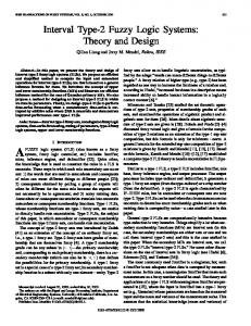
Fig. 1. Overview of the complete IT2 FLS composed by 𝐾 neurofuzzy filters [74].

(PSNR), and visual quality of the restored image. It is generally very difficult for a filter to produce both quantitatively excellent and visually satisfactory outputs. Regarding MGIN removal, Yang and Wu’s IPAMF+BM3D approach yields the best results from a visual quality perspective; while in the domain of pure impulse noise removal, an approach based on Interval Type-2 (IT2) TSK Fuzzy Logic System (FLS) [45], recently introduced by Yildirim et al. [74], has significantly exceeded all other filters in terms of quantitative measures. Based on the framework proposed by Yildirim et al. [74], this paper develops a Non-Singleton (NS) IT2 FLS1 [45], uses it jointly with the BM3D DCT filter, and shows that this new approach, referred to in the sequel as NS-IT2+BM3D, enables the highly corrupted images in MGIN environment to achieve excellent visual quality and exceptionally good quantitative results. The rest of the paper is organized as follows: Section II presents the overview of the complete FLS, the detailed structure of its building blocks, namely, the neurofuzzy filters, and how a training image set can be generated and used by a Quantum-behaved Particle Swarm Optimization (QPSO) algorithm to find the “optimal” set of design parameters for each neurofuzzy filter; Section III demonstrates the improved performance of our NS-IT2 FLS by comparing it against several other techniques as well as its T1 and singleton IT2 counterparts; Section IV draws conclusions for the paper. II. N OISE R EMOVAL BASED ON F UZZY L OGIC S YSTEM A. Neurofuzzy filters Our complete IT2 FLS has the general structure as depicted in Fig. 1. It is composed of 𝐾 neurofuzzy filters, each of which can be viewed as a sub-FLS, and has the same structure, 1 Compared

to Singleton FLSs, NS FLSs allow users to account for the uncertainties associated with the input measurements. Note that NS FLSs based on Gradient Descend Methods have been well studied in [45], but were never widely applied due to their extremely complicated gradient formulas. This paper shows how Quantum-behaved Particle Swarm Optimization algorithm enables designers to achieve “optimal” NS IT2-FLSs without having to derive the gradient formulas.

Fig. 3.

28 possible pixel topologies for the neurofuzzy filters [74].

i.e., the same number of antecedents, the same number of rules, and so on; but each uses a different input data set obtained from the given noisy image, and, therefore, has different design parameters. Each data set is obtained by shifting a 3 × 3 filtering window (see Fig. 2) through all pixels (excluding boundary pixels) in the image. Each time the window centers at a pixel, three of the nine pixels in the filtering window are selected to form an input vector, 𝒙𝑖 = [𝑥𝑖1 𝑥𝑖2 𝑥𝑖3 ]𝑇 (𝑖 = 1, . . . , 𝐾), for the 𝑖th neurofuzzy filter. Observe, in Fig. 3, that there are a total of 28 possible combinations of any three pixels in a filtering window, i.e., there can be at most 𝐾 = 28 neurofuzzy filters. To give a specific example, assume we are focusing on the 7th neurofuzzy filter that corresponds to pixel topology (7) in Fig. 3, and assume that the filtering window is centered at the pixel located at row 𝑟 and column 𝑐 (see Fig. 2), then the input vector for this neurofuzzy filter at this location is 𝒙7 = 𝑇 [𝑥71 𝑥72 𝑥73 ]𝑇 = [𝑥(𝑟 + 1, 𝑐 − 1) 𝑥(𝑟, 𝑐 − 1) 𝑥(𝑟, 𝑐)] . The output of this neurofuzzy filter is an interval of numbers of the noise-free luminance value at location (𝑟, 𝑐), 𝑌7 (𝑟, 𝑐) = [𝑦 7 (𝑟, 𝑐), 𝑦¯7 (𝑟, 𝑐)]. How the neurofuzzy filter actually obtains such an interval of numbers is described in details in Section II-B. A point-value for pixel (𝑟, 𝑐), 𝐷7 (𝑟, 𝑐), is then computed, as: 𝐷7 (𝑟, 𝑐) =

𝑦 7 (𝑟, 𝑐) + 𝑦¯7 (𝑟, 𝑐) 2

(1)

Similar operations are carried out by all other neurofuzzy filters, each using an input vector obtained based on the corresponding pixel topology. This leads to 𝐾 defuzzified values, 𝐷1 (𝑟, 𝑐), 𝐷2 (𝑟, 𝑐), . . . , 𝐷𝐾 (𝑟, 𝑐). A post-processor block takes these defuzzified values and performs the following

958

computations to obtain the final estimation, 𝑦ˆ(𝑟, 𝑐), of the noise-free luminance value at location (𝑟, 𝑐): 𝐾 1 ∑ 𝐷𝑖 (𝑟, 𝑐) 𝐷𝐴𝑉 (𝑟, 𝑐) = 𝐾 𝑖=1

⎧ 0  ⎨ 255 𝑦ˆ(𝑟, 𝑐) =  ⎩ round[𝐷

(2)

if 𝐷𝐴𝑉 (𝑟, 𝑐) < 0 if 𝐷𝐴𝑉 (𝑟, 𝑐) > 255 𝐴𝑉

(𝑟, 𝑐)]

(3)

otherwise

It is worth of mentioning that all the neurofuzzy filters can be computed in parallel to save computation time. B. Non-singleton Interval Type-2 Fuzzy Logic System 1) Structure: Type-2 (T2) FSs [46], [47], [81] have been shown to be more capable of modeling uncertainties than are T1 FSs. As a special case of T2 FSs, IT2 FSs have been widely used in FLS design for various applications [3], [4], [20], [44], [48]. On the other hand, a Non-Singleton (NS) FLS [45] allows users to take into consideration the uncertainties embedded in the input measurements, and gives the users more degree of design freedom by modeling input values as FSs instead of crisp numbers. In this paper, we build each of the neurofuzzy filters mentioned in Section II-A as a T1 NS IT2 FLS, where the input values are modeled as T1 FSs2 . Without loss of generality, assume we are focusing on the 𝑖th (𝑖 = 1, 2, . . . , 𝐾) neurofuzzy filter, and want to use it to obtain an interval estimation, 𝑌𝑖 (𝑟, 𝑐), of the pixel value at location (𝑟, 𝑐). Recall that the input vector is 𝒙𝑖 = [𝑥𝑖1 𝑥𝑖2 𝑥𝑖3 ], which is obtained by collecting three pixel values in the filtering window based on the corresponding topology. Our proposed NS IT2 FLS is based on 𝑁 rules that take the following forms: ˜ 𝑖2 is 𝐹˜ 1 and 𝑋 ˜ 𝑖3 is 𝐹˜ 1 ˜ 𝑖1 is 𝐹˜ 1 and 𝑋 Rule 1: IF 𝑋 𝑖1 𝑖2 𝑖3 1 ˜ THEN 𝑦𝑖 is 𝐺 𝑖 ⋅⋅⋅ ˜ 𝑖1 is 𝐹˜ 𝑁 and 𝑋 ˜ 𝑖2 is 𝐹˜ 𝑁 and 𝑋 ˜ 𝑖3 is 𝐹˜ 𝑁 Rule 𝑁 : IF 𝑋 𝑖1 𝑖2 𝑖3 𝑁 ˜ THEN 𝑦𝑖 is 𝐺 𝑖 ˜ 𝑘 (𝑘 = 1, ⋅ ⋅ ⋅ , 𝑁 ), is an where the consequent of each rule, 𝐺 𝑖 𝑘 ]; and IT2 FS whose centroid [33], [45] is the interval [𝑦𝑖𝑙𝑘 , 𝑦𝑖𝑟 each antecedent, 𝐹˜𝑖𝑗𝑘 (𝑗 = 1, 2, 3 and 𝑘 = 1, ⋅ ⋅ ⋅ , 𝑁 ), is an IT2 FS described by a Lower Membership Function (LMF) and an Upper Membership Function (UMF) that have the following forms, respectively (𝑢 ∈ 𝑋):

𝜇𝑘𝑖𝑗 (𝑢) =

⎧ ⎨ 𝑁 (𝑚𝑘𝑖𝑗 , 𝜎 𝑘 ; 𝑢) 𝑖𝑗

if 𝑢 ≤

⎩ 𝑁 (𝑚𝑘 , 𝜎 𝑘 ; 𝑢) 𝑖𝑗 𝑖𝑗

if 𝑢 >

⎧ 𝑘 𝑁 (𝑚𝑘𝑖𝑗 , 𝜎𝑖𝑗 ; 𝑢)  ⎨ 𝑘 1 𝜇𝑖𝑗 (𝑢) =  ⎩ 𝑁 (𝑚𝑘 , 𝜎 𝑘 ; 𝑢)

𝑘 𝑚𝑘 𝑖𝑗 +𝑚𝑖𝑗 2 𝑘 𝑚𝑘 𝑖𝑗 +𝑚𝑖𝑗 2

(4)

2 The input values can be further modeled as IT2 FSs, which will give the system even more degrees of design freedom, and has the potential to gain additional improvements for the performance. Since this paper is the first attempt to develop a NS IT2 FLS in the domain of image processing, and only has limited space, we only focus on the T1 NS IT2 FLS here, and will study the IT2 NS IT2 FLS in the future.

𝑖𝑗

𝑖𝑗

if 𝑢 < 𝑚𝑘𝑖𝑗

if 𝑚𝑘𝑖𝑗 ≤ 𝑢 ≤ 𝑚𝑘𝑖𝑗

(5)

if 𝑢 > 𝑚𝑘𝑖𝑗

𝑘 𝑘 𝑘 2 , 𝜎𝑖𝑗 ; 𝑢) = exp [− 12 (𝑢 − 𝑚𝑘𝑖𝑗 /𝜎𝑖𝑗 ) ]. Exwhere, e.g., 𝑁 (𝑚𝑖𝑗 th amples of the three antecedent IT2 FSs of the 𝑘 rule are depicted by the gray areas in Fig. 4, that are called Footprints Of Uncertainty (FOU). ˜ 𝑖𝑗 (𝑗 = 1, 2, 3), for the corresponding The input T1 FS, 𝑋 antecedent has the following MF (𝑢 ∈ 𝑋): 𝑘 𝜇𝑘𝑖𝑗 (𝑢) = 𝑁 (𝑥𝑖𝑗 , 𝜎𝑋 ˜ 𝑖𝑗 ; 𝑢)

(6)

where the mean of the MF is the actual crisp input value 𝑥𝑖𝑗 . Examples of the three input T1 FSs are depicted by the dotted lines in Fig. 4. 2) Inference Engine: Details regarding the above rule-based inference system can be found in [45], Chapter 11. This section briefly reviews all the necessary steps of the computations. First, the firing interval for every antecedent in each rule, 𝑘 [𝑓 𝑘𝑖𝑗 , 𝑓 𝑖𝑗 ] (𝑗 = 1, 2, 3 and 𝑘 = 1, 2, . . . , 𝑁 ), needs to be 𝑘

computed, where 𝑓 𝑘𝑖𝑗 (𝑓 𝑖𝑗 ) corresponds to the maximum value of the fuzzy intersections between the LMF (UMF) of 𝐹˜𝑖𝑗𝑘 and the MF of 𝑋𝑖𝑗 , respectively: ]} { [ 𝑓 𝑘𝑖𝑗 = max min 𝜇𝑘𝑖𝑗 (𝑢), 𝜇𝑘𝑖𝑗 (𝑢) (7) 𝑢∈𝑋

{ [ ]} 𝑘 𝑓 𝑖𝑗 = max min 𝜇𝑘𝑖𝑗 (𝑢), 𝜇𝑘𝑖𝑗 (𝑢)

(8)

𝑢∈𝑋

𝑘 An example of the fuzzy intersections between 𝜇𝑖𝑗 (𝑢) [𝜇𝑘𝑖𝑗 (𝑢)] 𝑘 th and 𝜇𝑖𝑗 for the 𝑘 rule are depicted by the heavy dashed (solid) 𝑘

lines in Fig. 4, where the corresponding 𝑓 𝑘𝑖𝑗 and 𝑓 𝑖𝑗 values are also labeled. Once the firing interval of each antecedent becomes avail𝑘 able, the firing interval for each rule, [𝑓𝑖𝑙𝑘 , 𝑓𝑖𝑟 ] (𝑘 = 1, 2, ⋅ ⋅ ⋅ , 𝑁 ), is obtained as follows: 𝑓𝑖𝑙𝑘 = 𝑘 𝑓𝑖𝑟 =

𝑗∈{1,2,3}

min

𝑓 𝑘𝑖𝑗

min

𝑓 𝑖𝑗

𝑗∈{1,2,3}

𝑘

(9) (10)

Finally, the Karnik-Mendel (KM) algorithm [33], [45] or the Enhanced KM (EKM) algorithm [69] is used to compute the following two values: ∑𝑁 𝑘 𝑘 𝑘=1 𝑓 𝑦𝑖𝑙 min (11) 𝑦 𝑖 (𝑟, 𝑐) = ∑ 𝑁 𝑘 ,𝑓 𝑘 ] 𝑘 𝑓 𝑘 ∈[𝑓𝑖𝑙 𝑖𝑟 𝑘=1 𝑓 ∑𝑁 𝑘 𝑘 𝑘=1 𝑓 𝑦𝑖𝑟 𝑦 𝑖 (𝑟, 𝑐) = max (12) ∑ 𝑁 𝑘 ,𝑓 𝑘 ] 𝑘 𝑓 𝑘 ∈[𝑓𝑖𝑙 𝑖𝑟 𝑘=1 𝑓 which are the desired outputs of the 𝑖th neurofuzzy filter, namely, 𝑌𝑖 (𝑟, 𝑐) at location (𝑟, 𝑐).

959

𝑘 (𝑢) and 𝜇𝑘 (𝑢), of the three antecedent IT2 FSs, 𝐹 ˜ 𝑘 (𝑗 = 1, 2, 3); the MFs, 𝜇𝑘 (𝑢), of the corresponding Fig. 4. An example of the LMFs and UMFs, 𝜇𝑖𝑗 𝑖𝑗 𝑖𝑗 𝑖𝑗 ˜ 𝑖𝑗 (𝑗 = 1, 2, 3); and, the fuzzy intersections between 𝜇𝑘 (𝑢) [𝜇𝑘 (𝑢)] and 𝜇𝑘 (𝑗 = 1, 2, 3), where (a) 𝑗 = 1; (b) 𝑗 = 2; (c) 𝑗 = 3. input T1 FSs , 𝑋 𝑖𝑗 𝑖𝑗 𝑖𝑗

Fig. 5. Training image set: (a) original image, and (b) image corrupted by 30% AWGN and 50% impulse noise.

For the above 𝑖th sub-system, each antecedent IT2 FS has 𝑘 , each input T1 FS has one three parameters, 𝑚𝑘𝑖𝑗 , 𝑚𝑘𝑖𝑗 and 𝜎𝑖𝑗 𝑘 parameter, 𝜎𝑋˜ , and each consequent has two parameters, 𝑦𝑖𝑙𝑘 𝑖𝑗 𝑘 and 𝑦𝑖𝑟 ; therefore, there are 3 × (3 + 1) + 2 = 14 parameters for each rule. We chose the number of rules3 to be 𝑁 = 33 = 27; consequently, the total number of parameters of each neurofuzzy filter is 𝑁 × 14 = 378. C. Training Image Set The training image set, which is used to tune the parameters of the neurofuzzy filters, consists of an original clean image and its corrupted version, and is artificially generated by a computer. The original image, depicted in Fig. 5(a), is 40 × 40 pixels and is divided into 10 × 10 = 100 boxes, i.e., each box contains 4 × 4 = 16 pixels. Pixels in each box have the same luminance value, an 8-bit integer uniformly distributed between 0 and 255. The corrupted image was obtained by adding MGIN to the original one. The noise level was carefully chosen because it has important impact on the performance of the entire system. After extensive simulations, we used 30% AWGN and 50% impulse noise to contaminate the clean image, and depict the corrupted output in Fig. 5(b). 3 𝑁 is chosen based on extensive simulations, where we tried to find an “optimal” number that provided satisfactory results and yet did not consume too much computation time.

To train the 𝑖th neurofuzzy filter, the filtering window shifted through all pixel locations (excluding the boundary pixels), i.e., 𝑟 = 2, 3, . . . , 𝑅 − 1 and 𝑐 = 2, 3, . . . , 𝐶 − 1, where 𝑅 and 𝐶 are the total number of rows and columns of the pixels in the given image; and a set of input vectors, 𝒙𝑖 , is collected. Then the rule-based inference system produce a set of 𝐷𝑖 (𝑟, 𝑐) values (𝑟 = 2, 3, . . . , 𝑅 − 1 and 𝑐 = 2, 3, . . . , 𝐶 − 1), which can be viewed as the 𝑖th neurofuzzy filter’s estimation of the original pixel values at corresponding locations. Note that all the neurofuzzy filters were trained independently; therefore, the post-processer block was not involved in this stage. The “optimal” set of design parameters is obtained by optimizing the Mean Square Error (MSE) of the estimated pixel values:

𝑀 𝑆𝐸 =

𝑅−1 ∑ 𝐶−1 ∑ 1 [𝐷𝑖 (𝑟, 𝑐) − 𝑦(𝑟, 𝑐)]2 (13) (𝑅 − 2)(𝐶 − 2) 𝑟=2 𝑐=2

where 𝑦(𝑟, 𝑐) is the original noise-free pixel value at (𝑟, 𝑐). Comment: A reviewer of this paper suggested that it is not very clear whether different images would need different training images. In response, we want to point out that only one training image set (as shown in Fig. 5) is needed to obtain a NS IT2 FLS that is universally applicable to all different images.■ D. Particle Swarm Optimization Different techniques can be employed to tune the parameters of the above neurofuzzy filters (NS IT2 FLSs), e.g., gradientbased methods [5], [21] proposed by Liang and Mendel [40], [45]. The analytical forms of the gradients of such a NS IT2 FLS that has this many parameters and nonlinear computations are quite complicated, making the computer implementation very difficult. In fact, this has been the main reason that has prevented NS T2 FLSs from becoming widely used. Also, the performance of the system can suffer significantly if the solution quickly falls into a local minimum, which can easily occur when gradient-based methods are used. In recent years, population-based random optimization techniques, such as Particle Swarm Optimization (PSO) [34], Genetic Algorithm (GA) [27] and evolutionary programming (EP) [22], have been widely applied to T1 FLS designs [14], [18], [23], [30]–[32], [41]. In this paper, we utilize the PSO

960

algorithm, because it is computationally fast, is the easiest to implement; and, as will be seen in Section III, it enables our system to provide very good results. 1) Quick Review: The standard PSO algorithm, first introduced by Kennedy and Eberhart [34], is briefly reviewed in this section4 . Let 𝑀 denote the swarm (population) size, where each particle in the swarm represents a possible solution to the optimization problem; 𝑛 denote the dimensionality of the search space; and, 𝐺 denote the total number of generations (iterations) of the optimization process. Each particle 𝑖 (𝑖 = 1, 2, . . . , 𝑀 ) has three inherent attributes: 1) a current position 𝑋 𝑖 = (𝑋𝑖,1 , 𝑋𝑖,2 , . . . , 𝑋𝑖,𝑛 ) in the search space; 2) a current velocity 𝑉 𝑖 = (𝑉𝑖,1 , 𝑉𝑖,2 , . . . , 𝑉𝑖,𝑛 ); and 3) a personal best (pbest) position (the position that produces the minimal value in the history of the particle) 𝑃 𝑖 = (𝑃𝑖,1 , 𝑃𝑖,2 , . . . , 𝑃𝑖,𝑛 ), i.e.: { if 𝑓𝑜𝑏𝑗 (𝑋 𝑖 (𝑡 + 1)) ≥ 𝑓 (𝑃 𝑖 (𝑡)) 𝑃 𝑖 (𝑡) 𝑃 𝑖 (𝑡+1) = 𝑋 𝑖 (𝑡 + 1) if 𝑓𝑜𝑏𝑗 (𝑋 𝑖 (𝑡 + 1)) < 𝑓 (𝑃 𝑖 (𝑡)) (14) where 𝑡 = 1, 2, . . . , 𝐺 − 1 is the index of generation. In each generation, each particle updates its velocity as follows (𝑗 = 1, 2, . . . , 𝑛; 𝑖 = 1, 2, . . . , 𝑀 ): 𝑉𝑖,𝑗 (𝑡 + 1) = 𝑤 ⋅ 𝑉𝑖,𝑗 (𝑡) + 𝑐1 ⋅ 𝑟1,𝑖 (𝑡)[𝑃𝑖,𝑗 (𝑡) − 𝑋𝑖,𝑗 (𝑡)] +𝑐2 ⋅ 𝑟2,𝑖 (𝑡)[𝑃𝑔,𝑗 (𝑡) − 𝑋𝑖,𝑗 (𝑡)] (15) where, e.g., 𝑋𝑖,𝑗 (𝑡) is the 𝑗 𝑡ℎ element of position of the 𝑖𝑡ℎ particle in the 𝑡𝑡ℎ generation; 𝑐1 and 𝑐2 are two constants called acceleration coefficients; 𝑟1,𝑖 (𝑡) and 𝑟2,𝑖 (𝑡) are two random variables uniformly distributed in the interval [0, 1]; 𝑤 is called inertia weight that is usually set to decrease linearly from 0.9 to 0.4 during the course of the search process to help PSO reach convergence; and, 𝑃 𝑔 (𝑡) denotes the global best (gbest) position found in the history of the entire swarm, i.e. (𝑖 = 1, 2, . . . , 𝑀 ): 𝑃 𝑔 (𝑡) = arg min 𝑓𝑜𝑏𝑗 (𝑃 𝑖 (𝑡)) 𝑃 𝑖 (𝑡)

𝑃 𝑖,𝑗 (𝑡 + 1) = 𝜂 × 𝑃 𝑖,𝑗 (𝑡) + (1 − 𝜂) × 𝑃 𝑔,𝑗 (𝑡)

(18)

where 𝜂 is a random variable uniformly distributed in (0, 1]; and 2) instead of using (17), the location of each particle is updated as:

(16)

At the end of each generation, a new position of a particle can be obtained, as: 𝑋 𝑖 (𝑡 + 1) = 𝑋 𝑖 (𝑡) + 𝑉 𝑖 (𝑡)

solution in the search space, and, they have shown that, in practice, the QPSO algorithm indeed provides better results for many widely-used benchmark tests than does the standard PSO algorithm. Therefore, this particular version of the PSO algorithm is our choice. Its pseudo-code is [70]: initialize 𝑋 𝑖 (1) (𝑖 = 1, . . . , 𝑀 ) randomly5 set 𝑃 𝑖 (1) = 𝑋 𝑖 (1) (𝑖 = 1, . . . , 𝑀 ) for 𝑡 = 1 to 𝐺 − 1 do ∑ 𝑀 1 calculate 𝑚(𝑡) = 𝑀 𝑖=1 𝑃 𝑖 (𝑡) 𝑃 𝑔 (𝑡) = arg min 𝑓𝑜𝑏𝑗 (𝑃 𝑖 (𝑡)) for 𝑖 = 1 to 𝑀 do if 𝑓 (𝑋 𝑖 (𝑡)) < 𝑓 (𝑃 𝑖 (𝑡)) then 𝑃 𝑖 (𝑡) = 𝑋 𝑖 (𝑡) end if for 𝑗 = 1 to 𝑛 do 𝜂 =rand(0,1) 𝑃 𝑖,𝑗 (𝑡 + 1) = 𝜂 × 𝑃 𝑖,𝑗 (𝑡) + (1 − 𝜂) × 𝑃 𝑔,𝑗 (𝑡) 𝑢 =rand(0,1) if rand(0,1)> 0.5 then 𝑋 𝑖,𝑗 (𝑡+1) = 𝑃 𝑖,𝑗 (𝑡+1)−𝛽∣𝑚𝑗 (𝑡)−𝑋 𝑖,𝑗 (𝑡)∣ ln 𝑢1 else 𝑋 𝑖,𝑗 (𝑡+1) = 𝑃 𝑖,𝑗 (𝑡+1)+𝛽∣𝑚𝑗 (𝑡)−𝑋 𝑖,𝑗 (𝑡)∣ ln 𝑢1 end if end for end for end for It can be seen that the QPSO algorithm differs from the PSO algorithm mainly in two ways: 1) instead of using (14), the best personal position of each particle is updated by taking a weighted average of its previous best personal and the global positions:

(17)

1 (19) 𝑢 where 𝑚(𝑡) is the average best personal positions of the entire swarm and 𝑢 is also a random variable uniformly distributed in (0, 1]. Note that (19) was developed based on the solution of the Schr¨odinger equation, which is why the algorithm has the prefix “Quantum-behaved”. 𝑋 𝑖,𝑗 (𝑡 + 1) = 𝑃 𝑖,𝑗 (𝑡 + 1) ± 𝛽∣𝑚𝑗 (𝑡) − 𝑋 𝑖,𝑗 (𝑡)∣ ln

2) Quantum-Behaved Particle Swarm Optimization: Despite its exceptionally good performance on many different problems, Van den Bergh [17] has shown that the PSO algorithm does not guarantee global optimization; therefore, ever since its debut in 1995, many variations and modifications of the PSO algorithm have been proposed to enhance its performance [38], [62], [82]. Recently, Sun et al [62], [70] proposed a Quantum-behaved PSO (QPSO) algorithm that, theoretically, guarantees optimal

Four widely used benchmark images (see Fig. 6) were chosen to test the performance of the above NS-IT2 FLS in comparison to median filter, Wiener filter, Gaussian filter, ROAD [25], and IPAMF+BM [73]. We also tested the T1 and singleton-IT2 counterparts of the proposed NS-IT2 FLS, as

4 Please distinguish the notations and labeling in this section from those in the previous section, as they are completely independent and denote different things here.

5 X (1) (𝑖 = 1, 2, . . . , 𝑀 ) are randomly initialized, because extensive 𝑖 simulations [62] have shown that the initial values of the locations have little impact on the convergence of the QPSO algorithm.

III. B ENCHMARK T ESTING

961

TABLE I MSE S OF DIFFERENT APPROACHES FOR THE FOUR BENCHMARK IMAGES ( BABOON , PENTAGON , BOAT, AND BRIDGE ) CORRUPTED BY 30% AWGN AND 30%, 50%, AND 70% IMPULSE NOISE , RESPECTIVELY Approach Median Filter Wiener Filter Gaussian Filter ROAD IPAMF+BM3D T1 FLS Singleton IT2 NS IT2 T1+BM3D Singleton-IT2+BM3D NS-IT2+BM3D

30% 5943.3 4015.6 5321.1 3085.3 5953.0 1936.6 1699.0 1633.7 1698.7 1391.1 1362.2

Baboon 50% 7173.5 3358.7 5942.5 4210.3 6720.1 2213.8 2062.8 2041.7 1747.2 1541.9 1532.1

70% 10269 3221.9 6902.4 5378.9 9461.9 2571.6 2498.5 2547.7 1916.3 1819.1 1847.1

30% 6163.7 4026.1 5445.4 3285.7 6575.0 1850.7 1433.5 1242.3 1493.7 1013.4 854.63

Pentagon 50% 7241.8 2962.0 5605.1 4898.9 7542.3 1800.4 1503.3 1335.5 1257.4 916.49 757.72

an effort to see whether modeling the inputs as FSs is indeed helpful. Three different levels of MGIN were generated for the test: 30% AWGN with 30%, 50%, and 70% impulse noise, respectively6 . The MSEs of the above techniques for the four images under different noise levels are summarized in Table I, where one can observe that, quantitatively, the fuzzy logic family (T1, singleton-IT2, and NS-IT2 FLSs) significantly out-performed the other techniques. In addition, after extensive simulations, it was found that the performance of the fuzzy logic family can 6 Due to page limit, we only tested a limited number of different noise levels; therefore, it remains as an open issue how much noise must be present before the NS IT2 FLS provides a significant improvement over the singleton IT2 FLS.

Fig. 6. Four benchmark test images: (a) baboon; (b) pentagon; (c) boat; (d) bridge.

70% 9933.5 2376.2 6058.1 5571.4 9214.9 1813.6 1600.0 1502.8 1121.4 889.19 771.88

30% 6042.5 4271.4 5676.3 2844.0 6069.0 2124.6 1874.0 1778.8 1742.9 1431.6 1367.1

Boat 50% 7231.7 3531.3 6167.6 3928.6 6753.1 2383.2 2214.4 2124.1 1810.5 1594.9 1518.1

70% 10330 3303.8 7003.4 4965.4 8591.7 2779.2 2637.5 2565.6 2066.0 1902.5 1816.2

30% 5934.5 4861.2 6152.7 2878.8 5991.6 2817.3 2479.2 2481.9 2512.0 2125.9 2157.4

Bridge 50% 7260.2 4468.2 6899.4 3935.2 8096.1 3338.4 3055.4 3013.3 2844.1 2510.9 2473.0

70% 10682 4401.1 7934.6 4953.4 11506 4006.4 3737.2 3595.0 3343.1 3045.7 2885.8

be greatly enhanced when used jointly the with BM3D7 DCT filter [16], which is a fast way to remove the residual AWGN after the FLS process. The MSEs of such joint approaches between fuzzy logic family and BM3D are also given in Table I, where one can observe that the NS-IT2+BM3D approach generally out-performs other techniques and its T1 and singleton-IT2 counterparts, with noticeable improvements, except in two cases, image “Baboon” with 70% impulse noise 7 The implementations of the BM3D filter has been generously made available online by its authors [16]. But since it is just a complement to our technique and is not the focus of this paper, the details of BM3D are not provided here.

Fig. 7. (a) Image “boat” corrupted by 30% AWGN and 50% impulse noise; and its restored versions based on (b) median filter; (c) Wiener filter; (d) Gaussian filter; (e) ROAD; (f) IPAMF+BM3D; (g) T1+BM3D; (h) singletonIT2+BM3D; (i) NS-IT2+BM3D

962

TABLE II AVERAGE MSE S OF THE FOUR BENCHMARK IMAGES FOR DIFFERENT APPROACHES UNDER 30% AWGN AND 30%, 50%, AND 70% IMPULSE NOISE , RESPECTIVELY Median Filter Wiener Filter Gaussian Filter ROAD IPAMF+BM3D T1 FLS Singleton IT2 NS IT2 T1+BM3D Singleton-IT2+BM3D NS-IT2+BM3D

30% 6021.0 4293.6 5648.9 3023.5 6147.2 2182.3 1871.4 1784.2 1861.8 1490.5 1435.4

50% 7226.8 3580.1 6153.7 4243.3 7277.9 2434.0 2209.0 2128.7 1914.8 1641.0 1570.2

70% 10303 3325.8 6974.6 5217.3 9693.6 2792.7 2618.3 2552.8 2111.7 1914.1 1830.2

and “Bridge” with 30% impulse noise, where the singletonIT2+BM3D has slightly better results. To give an overview of these results, the average MSEs of the four images are summarized in Table II, where we can observe that the NSIT2+BM3D always out-performs other techniques in terms quantitative measures. Fig. 7 presents the image “boat” corrupted by 30% AWGN and 50% impulse noise and its restored versions based on the above techniques. Observe that the NS-IT2+BM3D appear to give the best visual restoration. Similar results were obtained for other images and under other noise levels. IV. C ONCLUSION This paper presented a NS-IT2 FLS framework for removing MGIN from digital images. Using only one set of artificially generated training images, the design parameters of the system were tuned by a QPSO algorithm which allowed us to avoid using complex gradient-descent methods. The paper showed that the proposed technique yields both quantitatively and visually much better results compared to several widelyused non-fuzzy noise removal filters. Also, by introducing more degrees of design freedom into the system, the NS-IT2 FLS has also been shown to out-perform its T1 and singletonIT2 counterparts. R EFERENCES [1] E. Abreu, M. Lightstone, S. K. Mitra, and K. Arakawa. A new efficient approach for the removal of impulse noise from highly corrupted images. IEEE Trans. on Image Processing, 5(6):1012–1025, June 1996. [2] I. Aizenberg, C. Butakoff, and D. Paily. Impulsive noise removal using threshold Boolean filtering based on the impulse detecting functions. IEEE Signal Processing Letter, 12(1):63–66, 2005. [3] L. Astudillo, O. Castillo, and L. T. Aguilar. Intelligent control for a perturbed autonomous wheeled mobile robot: a type-2 fuzzy logic approach. Journal of Nonlinear Studies, 14(3):37–48, 2007. [4] P. Baguley, T. Page, V. Koliza, and P. Maropoulos. Time to market prediction using type-2 fuzzy sets. Journal of Manufacturing Technology Management, 17(4):513–520, 2006. [5] D. Bertsekas. Nonlinear Programming. Athena Scientific, Belmont, Massachusetts, second edition, 1999. [6] E. Besdok, P. C¸ivicio glu, and M. Alc¸i. Impulsive noise suppression from highly corrupted images by using resilient neural networks. Lecture Notes in Computer Science, 3070:670–675, 2004. [7] E. Besdok and M. E. Y¨uksel. Impulsive noise rejection from images with jarque-berra test based median filter. International Journal of Electronics and Communications, 59(2):105–109, 2005.

[8] R. H. Chan, C. Hu, and M. Nikolova. An iterative procedure for removing random-valued impulse noise. IEEE Signal Processing Letter, 11(12):921–924, 2004. [9] J. Y. Chang and J. L. Chen. Classifier augmented median filter for image restoration. IEEE Trans. on Instrumentation and Measurement, 53(2):351–356, 2004. [10] T. Chen, K. K. Ma, and L. H. Chen. Tri-state median filter for image denoising. IEEE Trans. on Image Processing, 8(12):1834–1838, 1999. [11] T. Chen and H. R. Wu. Adaptive impulse detection using centerweighted median filters. IEEE Signal Processing Letter, 8(1):1–3, 2001. [12] T. Chen and H. R. Wu. Space variant median filters for the restoration of impulse noise corrupted images. IEEE Trans. on Circuits and Systems, 48(8):784–789, 2001. [13] Y. S. Choi and R. Krishnapuram. A robust approach to image enhancement based on fuzzy logic. IEEE Transactions on Image Processing, 6(6):808–825, June 1997. [14] O. Cordon, F. Gomide, F. Herrera, F. Hoffmann, and L. Magdalena. Ten years of genetic fuzzy systems: current framework and new trends. Fuzzy Sets and Systems, 141(1):5–31, 2003. [15] V. Crnojevic, V. Senk, and Z. Trpovski. Advanced impulse detection based on pixel-wise MAD. IEEE Signal Processing Letter, 11(7):589– 592, 2004. [16] K. Dabov, A. Foi, V. Katkovnik, and K. Egiazarian. Image denoising by sparse 3D transform-domain collaborative filtering. IEEE Trans. on Image Processing, 16(8):2080–2095, August 2007. [17] F. Van den Bergh. An analysis of particle swarm optimizer. PhD thesis, University of Pretoria, Pretoria, South Africa, 2001. [18] L. dos Santos Coelho and B. M. Herrera. Fuzzy identification based on a chaotic particle swarm optimization approach applied to a nonlinear yoyo motion system. IEEE Trans. on Industrial Electronics, 54(6):3234– 3245, 2007. [19] H.-L. Eng and K.-K. Ma. Noise adaptive soft-switching median filter. IEEE Trans. on Image Processing, 10(2):242–251, February 2001. [20] H. Rhee F. C. Uncertainty fuzzy clustering: insights and recommendations. IEEE Computational Intelligence Magazine, 2(1):44–56, 2007. [21] R. Fletcher. Practical Methods of Optimization. Wiley, Hoboken, New Jersey, second edition, 2000. [22] L. J. Fogel. Evolutionary programming in perspective: the top-down view. In J. M. Zurada, R. J. Marks II, and C. J. Robinson, editors, Computational Intelligence: Imitating Life. IEEE Press, Piscadaway, NJ, 1994. [23] A. Fowler, A. M. Teredesai, and M. De Cock. An evolved fuzzy logic system for fire size prediction. In Proc. of The 28th North American Fuzzy Information Processing Society Annual Conference (NAFIPS 2009), pages 1–6, Cincinnati, OH, 2009. [24] M. Gabbouj, E. J. Coyle, and N. C. Gallager. An overview of median and stack filtering. Circuits, Systems, and Signal Processing, 11(1):7–45, 1992. [25] R. Garnett, T. Huegerich, and C. Chui. A universal noise removal algorithm with an impulse detector. IEEE Transactions on Image Processing, 14(11):1747–1754, November 2005. [26] R. Garnett, T. Huegerich, C. Chui, and W. He. A universal noise removal algorithm with an impulse detector. IEEE Trans. on Image Processing, 14(11):105–109, 2005. [27] D. E. Goldberg. Genetic Algorithms in search Optimization and Machine Learning. Addison-Wesley, Reading, Massachusetts, 1989. [28] R. Gonzalez and R. E. Woods. Digital Image Processing. Prentice Hall, Upper Saddle River, New Jersey, third edition, 2007. [29] W. Y. Han and J. C. Lin. Minimum-maximum exclusive mean filter to remove impulse noise from highly corrupted images. Electronic Letters, 33(2):124–125, 1997. [30] F. Hoffmann. Evolutionary algorithms for fuzzy control system design. Proceedings of the IEEE, 89(9):1318–1333, 2001. [31] C. F. Juang. A tsk-type recurrent fuzzy network for dynamic systems processing by neural network and genetic algorithms. IEEE Trans. on Fuzzy Systems, 10(2):155–170, 2002. [32] C. F. Juang, C. M. Hsiao, and C. H. Hsu. Hierarchical cluster-based multispecies particle-swarm optimization for fuzzy-system optimization. IEEE Trans. on Fuzzy Systems, 18(1):14–26, 2010. [33] N. N. Karnik and J. M. Mendel. Centroid of a type-2 fuzzy set. Information Sciences, 132:195–220, 2001. [34] J. Kennedy and R. Eberhart. Paticle swarm optimization. In Proceedings of IEEE International Conference on Neural Networks, pages 1942– 1948, Perth, WA , Australia, 1995.

963

[35] C. Kenney, Y. Deng, B. S. Manjunath, and G. Hewer. Peer group image enhancement. IEEE Transactions on Image Processing, 6(2):326–334, February 2001. [36] V. V. Khryashchev, I. V. Apalkov, A. L. Priorov, and P. S. Zovanarev. Image denoising using adaptive switching median filter. In IEEE Internation Conference on Image Processing, pages 117–120, Genoa, Italy, 2005. [37] S. J. Ko and Y. H. Lee. Center weighted median filters and their applications to image enhacement. IEEE Trans. on Circuits and Systems, 38(9):984–993, 1991. [38] R. A. Krohling and L. dos Santos Coelho. Coevolutionary particle swarm optimization using gaussian distribution for solving constrained optimization problems. IEEE Trans. on Systems, Man, and Cybernetics, Part B: Cybernetics, 36(6):1407–1416, 2006. [39] C.-S. Lee, Y.-H. Kuo, and P.-T. Yu. Weighted fuzzy mean filter for image processing. Fuzzy Sets and Systems, 89(2):157–180, 1999. [40] Q. Liang and J. M. Mendel. Interval type-2 fuzzy logic systems: Theory and design. IEEE Trans. on Fuzzy Systems, 8:535–550, 2000. [41] B. D. Liu, C. Y. Chen, and J. Y. Tsao. Design of adaptive fuzzy logic controller based on linguistic-hedge concepts and genetic algorithms. IEEE Trans. on Systems, Man, and Cybernetics, Part B: Cybernetics, 31(1):32–53, 2001. [42] W. Luo. An efficient detail-preserving approach for removing impulse noise in images. IEEE Signal Processing Letters, 13(7):413–416, July 2006. [43] Z. Ma, H. R. Wu, and B. Qiu. An robust structure adaptive hybrid vector filter for color image restoration. IEEE Transactions on Image Processing, 14(12):1900–2001, December 2005. [44] P. Melin, J. Urias, D. Solano, M. Soto, M. Lopez, and O. Castillo. Voice recognition with neural networks, type-2 fuzzy logic and genetic theory. Information Sciences, 13(2):108–116, 2006. [45] J. M. Mendel. Uncertain Rule-Based Fuzzy Logic Systems: Introduction and New Directions. Prentice-Hall, Upper Saddle River, NJ, 2001. [46] J. M. Mendel and R. I. John. Type-2 fuzzy sets made simple. IEEE Trans. on Fuzzy Systems, 10(2):117–127, 2002. [47] J. M. Mendel, F. Liu, and D. Zhai. Alpha-plane representation for type2 fuzzy sets: theory and applications. IEEE Trans. on Fuzzy Systems, 17(5):1189–1207, 2009. [48] J. M. Mendel and D. Wu. Perceptual Computing: Aiding People in Making Subjective Judgements. Wiley-IEEE Press, Hoboken, New Jersey, 2010. [49] S. Morillas, V. Gregori, G. Peris-Fajarne, and P. Latorre. A fast impulsive noise color image filter using fuzzy metrics. Real-Time Imaging, 11(5):417–428, 2005. [50] P. Perona and J. Malik. Scale-space and edge detection using anisotropic diffusion. IEEE Trans. on Pattern Analysis and Machine Intelligence, 12(5):629–639, May 1990. [51] K. N. Plataniotis and A. N. Venetsanopoulos. Color Image Processing and Applications. Springer, Heidelberg, Germany, first edition, 2000. [52] K. N. Plataniotis, S. Vinayagamoorthy, D. Androutsos, and A. N. Venetsanopoulos. An adaptive nearest neighbor multichannel filter. IEEE Transactions on Circuits and Systems for Video Technology, 6(6):699– 703, December 1996. [53] G. Pok, Y. Liu, and A. S. Nair. Selective removal of impulse noise based on homogeneity level information. IEEE Trans. on Image Processing, 12(1):85–92, 2003. [54] S. M. M. Rahman and M. K. Hasan. Wavelet-domain iterative center weighted median filter for image denoising. Signal Processing, 83(5):1001–1012, 2003. [55] F. Russo. Fire operators for image processing. Fuzzy Sets and Systems, 103(2):265–275, 1999. [56] F. Russo. Noise removal from image data using recursive neurofuzzy filters. IEEE Transactions on Instrumentation and Measurement, 49(2):307–314, April 2000. [57] F. Russo. Impulse noise cancellation in image data using a two-output nonlinear filter. Measurement, 36:205–213, 2004. [58] F. Russo and G. Ramponi. A fuzzy filter for image corrupted by impulse noise. IEEE Signal Processing Letters, 3(6):168–170, June 1996. [59] S. Schulte, M. Nachtegael, V. De Witte, D. Van der Weken, and E. E. Kerre. A fuzzy impulse noise detection and reduction method. IEEE Trans. on Image Processing, 15(5):1153–1162, May 2006. [60] B. Smolka and A. Chydzinski. Fast detection and impulsive noise removal in color images. Journal of Real-Time Image Processing, 11(4):389–402, 2005.

[61] B. Smolka, K. N. Plataniotis, A. Chydzinski, M. Szczepanski, A. N. Venetsanopulos, and K. Wojciechowski. Self-adaptive algorithm of impulsive noise reduction in color images. Pattern Recognition, 35(8):1771–1784, 2002. [62] J. Sun, W. B. Xu, and B. Feng. A global search strategy of quantumbehaved particle swarm optimization. In Proc. of 2004 IEEE Conference on Cybernetics and Intelligent Systems, pages 111–116, 2004. [63] T. Sun and Y. Neuvo. Detail-preserving median based filters in image processing. Pattern Recognition Letter, 15(4):341–347, 1994. [64] C. Tomasi and R. Manduchi. Bilateral filtering for gray and color images. In Proc. of IEEE International Conference on Computer Vision, Bombay, India, 1998. [65] S. E. Umbaugh. Computer Vision and Image Processing: A Practical Approach using CVIPTools. Prentice Hall, Upper Saddle River, NJ, 1998. [66] D. Van De Ville, M. Nachtegael, D. Van der Weken, E. E. Kerre, W. Philips, and I. Lemahieu. Noise reduction by fuzzy image filtering. IEEE Transactions on Fuzzy Systems, 11(4):429–436, August 2003. [67] Z. Wang and D. Zhang. Progressive switching median filter for the removal of impulse noise from highly corrupted images. IEEE Trans. on Circuits and Systems, 46(1):78–80, 1999. [68] P. S. Windyga. Fast impulsive noise removal. IEEE Transactions on Image Processing, 10(1):173–179, 2001. [69] D. Wu and J. M. Mendel. Enhanced Karnik - Mendel algorithms. Information Sciences, 17(4):923–934, 2009. [70] M. Xi, J. Sun, and W. Xu. An improved quantum-behaved particle swarm optimization algorithm with weighted mean best position. Applied Mathematics and Computation, 205:751–759, 2008. [71] H. Xu, G. Zhu, H. Peng, and D. Wang. Adaptive fuzzy switching filter for images corrupted by impulse noise. Pattern Recognization Letters, 25(15):1657–1663, November 2004. [72] N. Yamashita, M. Ogura, J. Lu, H. Sekiya, and T. Yahagia. Random valued impulse noise detector using level detection. In IEEE International Symposium on Circuits and Systems, pages 6292–6295, Kobe, Japan, 2005. [73] J.-X. Yang and H.-R. Wu. Mixed Gaussian and uniform impulse noise analysis using robust estimation for digital images. In 16th International Conference on Digital Signal Processing, pages 1–5, Santorini-Hellas, 2009. [74] M. T. Yildirim, A. Bast¨urk, and M. E. Y¨uksel. Impulse noise removal from digital images by a detail-preserving filter based on type-2 fuzzy logic. IEEE Transactions on Fuzzy Systems, 16(4):920–928, 2008. [75] L. Yin, R. Yang, M. Gabbouj, and Y. Neuvo. Weighted median filters: A tutorial. IEEE Trans. on Circuits and Systems II, 43(3):157–192, 1996. [76] O. Yli-Harja, J. Astola, and Y. Neuvo. Analysis of the properties of median and weighted median filters using threshold logic and stack filter representation. IEEE Trans. on Signal Processing, 39(2):395–410, 1991. [77] S. Q. Yuan and Y. H. Tan. Impulse noise removal by a global-local noise detector and adaptive median filter. Signal Processing, 86(8):2123–2128, 2006. [78] M. E. Y¨uksel. A hybrid neuro-fuzzy filter for edge preserving restoration of images corrupted by impulse noise. IEEE Trans. on Image Processing, 15(4):928–936, April 2006. [79] M. E. Y¨uksel and A. Bast¨urk. Efficient removal of impulse noise from highly corrupted digital images by a simple neuro-fuzzy operator. International Journal of Electronics and Communications, 57(3):214– 219, 2003. [80] M. E. Y¨uksel and E. Besdok. A simple neuro-fuzzy impulse detector for efficient blur reduction of impulse noise removal operators for digital images. IEEE Trans. on Fuzzy Systems, 12(6):854–865, December 2004. [81] D. Zhai and J. M. Mendel. Uncertainty measures for general type-2 fuzzy sets. Information Sciences, In Press. [82] Z. H. Zhan, J Zhang, Y. Li, and H. S.-H. Chung. Adaptive particle swarm optimization. IEEE Trans. on Systems, Man, and Cybernetics, Part B: Cybernetics, 39(6):1362–1381, 2009. [83] S. Zhang and M. A. Karim. A new impulse detector for switching median filters. IEEE Signal Processing Letter, 9(11):360–363, 2002.

964