() 1994 Society for Industrial and Applied Mathematics
SIAM J. ScI. COMPUT.
Downloaded 04/22/14 to 128.135.149.17. Redistribution subject to SIAM license or copyright; see http://www.siam.org/journals/ojsa.php
Vol. 15, No. 1, pp. 207-224, January 1994
014
A NONLINEAR VARIATIONAL PROBLEM FOR IMAGE MATCHING* YALI AMITt Abstract. Minimizing a nonlinear functional is presented as a way of obtaining a planar mapping that matches A smoothing term is added to the nonlinear functional to penalize discontinuous and irregular solutions. One option for the smoothing term is a quadratic form generated by a linear differential operator. The functional is then minimized using the Fourier representation of the planar mapping. With this representation the quadratic form is diagonalized. Another option is a quadratic form generated via a basis of compactly supported wavelets. In both cases, a natural approximation scheme is described. Both quadratic forms are shown to impose the same smoothing. However, in terms of the finite dimensional approximations, it is easier to accommodate local deformations using the wavelet basis. two similar images.
Key
words,
image matching, movement compensation, nonlinear variational problem, spectral methods,
wavelets
AMS subject classifications. 68V10, 65M70, 49N60
1. Introduction. Let F and G be smooth functions on the two-dimensional unit square
12, and let 4(x) be a mapping of the unit square into itself, such that G(x)
F(4(x)). It is
clear that if F and G have the same range, many such mappings exist, most of which would be highly discontinuous and degenerate and not very interesting. However, if the mapping q (x) is a smooth diffeomorphism of the unit square onto itself, then the extremal points of F would be mapped via 4-1 onto the extremal points of G, level curves would be mapped onto level curves, etc. Heuristically speaking, the graphs of F and G considered as surfaces would have similar topographies. Conversely, if F and G have similar topographies, then it should be possible to find a smooth and locally nondegenerate mapping q such that F((x)) is close to G in some sense. To illustrate this idea, consider the images in Fig. 1, which are x-rays of two different hands. If we consider the images as some smooth function sampled at the points of the pixel lattice, we obtain two functions that indeed have very similar topographies. This would be the case with any two images of some fixed organ of the body of two different patients, or of the same patient obtained at different times, provided that these images came from the same type of imaging device. Consequently, there should exist a smooth and locally nondegenerate mapping q that transforms one image, called the template, into the other image, called the data, via composition. The mapping q would automatically match between the corresponding parts of the two images. See, for example, Fig. 1 where the various parts of the hand such as the tips of the fingers or the joints are correctly matched. One ofthe first attempts dealing with the issue of image matching can be traced to Horn and Schnuck [5] and Huang and Tsai [6] in the context of optical flow and movement compensation calculations for sequences of images. These ideas were further developed by Nagel 10] and Terzopoulos 11]. In Bajcy and Kovacic [2] these ideas were applied to the issue of matching medical images of similar organs, such as MRI images of the brain. Here the matching is not intended to calculate movement, but to automate the analysis of medical images. This second problem is also more difficult in that large deformations may occur, as opposed to relatively small deformations in image sequences. *Received by the editors April 1, 1991; accepted for publication (in revised form) March 1, 1993. This research was supported in part by Office of Naval Research grant N00014-88-K-0289 and Army Research Office grant
DAAL03-90-G-0033. fDepartment of Statistics, University of Chicago, Chicago, Illinois 60637. This work was done while the author was at Brown University, Division of Applied Mathematics, Providence, Rhode Island 02912 (
[email protected]). 207
Downloaded 04/22/14 to 128.135.149.17. Redistribution subject to SIAM license or copyright; see http://www.siam.org/journals/ojsa.php
208
YALI AMIT
Tern
] ate
Restoration
Final Difference
Initial Di ierence
Data
Restoration
Di splacement Field
FIG. 1. The template corresponds to the function F and the data to the function G. The restoration was done using the Fourier method. The white lines show the matching induced by the displacement field. A point x in the data is connected via the restoration to the point x -t- U (x) from which it obtained its grey level value. The final difference image shows IF(x + U(x)) G(x)] and the initial difference image shows IF(x) G(x)l.
-
The question is how to find the mapping b. We have addressed this problem by minimizing the following functional:
(1)
I(U)
IF(x
+ U(x)) G(x)12dx,
where U(x) qb(x) x is the displacement field and T 2 is the unit torus. Minimizing I over some set of vector fields provides a mapping b (x) x -t- U(x) of the torus into itself, such that F o 4 (x) is close in the mean square norm to G. It should be noted that the periodic domain is chosen for the sake of notational and computational convenience. It takes care of the problem of what to do when x -t- U(x) is not
Downloaded 04/22/14 to 128.135.149.17. Redistribution subject to SIAM license or copyright; see http://www.siam.org/journals/ojsa.php
VARIATIONAL PROBLEM FOR IMAGE MATCHING
209
in 12. Another possibility is that F is defined on some large domain D that includes 12. Then one would want to minimize over mappings from I 2 into D. To rule out the discontinuous and irregular solutions to this minimization problem, it is possible to introduce a smoothing or regularizing term, thus obtaining a new functional
(2)
J(U)
orS(U, U) -k-
-
IF(x q- U(x))
G(x)12dx,
where is a bilinear form penalizing nonsmooth functions. In all our applications, was taken to be a Hilbertian norm equivalent to one of the Sobolev norms. Since the domain under consideration is two dimensional, taking the Sobolev norm to be of order greater or equal to two will ensure that the solutions are continuous. Higher-order Sobolev norms will, of course, introduce additional smoothness. This approach was first described in a statistical setting by Amit, Grenander, and Piccioni 1 ]. The functional J is nonlinear and may have many global and local minima. In the sequel we will be interested mainly in finding local minima of J close to the initialpoint U(x) 0 that corresponds to the identity map. The nondegeneracy of the mapping q generated by a local minimizer is then ensured by the fact that it is close to the identity map so that its Jacobian is nonzero at most points. There are several major differences between the work mentioned above and the approach presented here. First, we do not use a data term derived from intensity conservation assumptions originally suggested by Horn and Schnuck [5], which is equivalent to linearizing the functional I as described at the end of 2. It appears that the linearized problem will not capture larger deformations (see Fig. 2). Second, the solution of the variational problem is obtained by parametrizing the unknown function in terms of its coefficients with respect to either the Fourier basis or some wavelet basis, thus allowing for a coarse-to-fine or multiresolution approach. This was indeed suggested in 11 using multigrid techniques, which may be appropriate for the linearized equations that have a unique solution and are known to be efficiently soluble using multigrid techniques. However, given that the nonlinear functional is to be used, and that this nonlinear functional is not convex, it is not clear how well the classical multigrid approach will perform. The coarse level displacement is calculated using only the information of a smooothed version of the data on that same coarse grid, and there is some risk of information being lost. Moreover, when moving to finer grids, a bilinear interpolation is used that may not be smooth enough and that may introduce unnatural deformations. Setting the problem in terms of an orthonormal basis directly incorporates interpolation through the basis functions. The smoothing operator is automatically written in diagonal form in terms of the basis chosen. Thus using the description in terms of a basis expansion, and solving first for low-frequency coefficients, gradually increasing the number can be thought of as a multigrid method translated onto the finest grid. Although some computational speed is lost, the advantage is that all the data is used to drive the algorithm. The level of smoothness versus locality can be controlled by the choice of wavelet basis. Since the problem at hand is not really governed by physical fluid dynamical or elasticity laws, there is no special advantage in using the Laplacian as a smoothing operator. The existence of fast transforms for these bases makes the algorithm computationally feasible. In 2 the smoothing term g is set to be a quadratic form generated by a linear differential operator. The approximations are then described together with minimization procedure. The basic idea is to diagonalize the differential operator using the Fourier basis and to solve the problem in the spectral domain.
210
YALI AMIT
Downloaded 04/22/14 to 128.135.149.17. Redistribution subject to SIAM license or copyright; see http://www.siam.org/journals/ojsa.php
Temp ae
Restoration
Temp ate
Data
Restoration
Data
Di splacement Field
Di splacement Field
(b)
(a)
(c) FI. 2. A transformation constructed with the Fourier basis was initially applied to the template to generate the data. (a) was done using the Fourier basis. (b) was done using the wavelet basis. (c) was done using the linearized equations.
211
VARIATIONAL PROBLEM FOR IMAGE MATCHING
Downloaded 04/22/14 to 128.135.149.17. Redistribution subject to SIAM license or copyright; see http://www.siam.org/journals/ojsa.php
In 3 an alternative smoothing term is suggested. This time
is directly given in a The the Fourier basis. eigenvalues are set so diagonal form using a wavelet basis instead of as to ensure the same type of smoothing. In 4 the experiments are described, and the performance of the two approaches is com-
pared. 2. A nonlinear partial differential equation. Consider the bilinear form
B(f, g)
1
fr2(A + )2
e f(x). g(x)dx,
where A denotes the Laplacian with periodic boundary conditions. This bilinear form defines a Hilbertian norm equivalent to the standard Sobolev norm on H H2(T2). Set s(U, U) B(U (1), U (1)) + B(U (2), U (2)) in (2). With this choice of the bilinear form in the functional J, the Euler equation for the minimizer is the following nonlinear partial differential equation
(PDE): O(t o/(t
-
OF
E)2U (1)
(G(x)
F(x
+ U(x)))-x, (X + U(x)),
+ 8)2U (2)
(G(x)
F(x
r- U(x)))-x2(X + U(x)).
OF
The parameter a determines the relative weight of the regularizing term. Since the issue of the 1. This is the parameter used in the experiments choice of is not addressed here, we set ot as well. For the purpose of numerical solutions, it is, of course, necessary to find finite-dimensional approximations to the functional J. Since the spectral decomposition of A is known, it is convenient to write J in the spectral domain and then approximate it coordinatewise. Let )kt, kl denote the eigenvalues and eigenvectors of A, then
kl
(2:rt’)2(k2 + 12) + e
and (kl(Xl, X2)
e2ri(kx+tx2),
and the functional J can be rewritten as --2
J(U)
(1),2
AklttUkl
+
(2).2.
Ukl
k,l=-x
+
(2)
a(x)] dx
F(u(1), u (2)) + q(u (1),/1(2)), where Ukl(i)
The vector (u (1) u (2)) e2 e2, is simply the coordinate vector of (U (1), U (2)) with respect to the basis t of L2(T2). We write (u (1), u (2)) zr(U (1), U()). Note that q(u (1), u ()) I(U (1), U (2)) with I as in (1). The finite dimensional approximations of the functional are obtained by taking the sums in the linear term and those in the integrand between -(N 1) and N. The approximation is therefore obtained by restricting the argument of J to the space HN HN, where Hv sPan{dflkl}ff.l=_(N_l). The dimension of the approximate space Hv is (2N) z and zr(Hv x
f u(i)(x)cp/d(x)dx.
HN)-- R (2N)2 R (2N)2. Let Jv denote the approximate functional on Hv x HN. Each of the finite dimensional as U o and therefore has functionals is positive and continuous. Moreover, Jv (U) at least one global minimum. Let Sv be the set of global minima of Jv.
Downloaded 04/22/14 to 128.135.149.17. Redistribution subject to SIAM license or copyright; see http://www.siam.org/journals/ojsa.php
212
YALI AMIT
THEOREM. Let UN SN for N 1, 2 Then UN has a convergent subsequence in H x H, which converges to a global minimum of J. Proof. Consider H x H with the Hilbertian norm defined by g(.,-). Since H x H is compactly imbedded in C(T 2) x C(T2), IUN UIHH --+ 0 implies uniform convergence that, in turn, implies that G (x + UN (x)) -+ G (x + U(x)), as N cxz. Since G and F are bounded, it follows from the dominated convergence theorem that I(UN) -+ I(U). Clearly, (UN, UN) (U, U), so that J is continuous in H. Now JN (UN) is a positive monotonically decreasing sequence so that it converges to some value L. Moreover, since UN is the global minimum of J in HN x HN, and since k/= (HN x HN) is dense in H x H, it follows from the continuity of J that L infunn J(U). Since UNIH n the sequence (UN, UN) < Jm (UN) < J1 (U1) for all N 1, 2 is Let be a that to U H x H. weakly some compact. subsequence converges weakly UN Umk Again, since H is compactly embedded in C (T2), UNk converges in the uniform norm to U as k o. As above, this implies that I (UN) -+ I (U). Together with the fact that J(UN) converges, we conclude that (UN, UN) converges to L [ (U) as k --+ o. Now since the norm function is lower semicontinuous in the weak topology, we have g(U, U) r log 2 R + 1 there are at most two terms in the sum. P cannot be expressed as scales and shifts of For small n the functions apnk P0 (x) _= P e However, for n > r, we have p (n+l)k(x) VCn(2X --k), where the argument is considered modulo 1 or on the unit circle. Moreover, the family of functions pe and 0, 1 nk for n
e
217
VARIATIONAL PROBLEM FOR IMAGE MATCHING
1 form an orthonormal basis. Let 1 together with the function q0 V0 span{40} (i.e., the constant functions) and Wn span{ "t’Pv,nk}2"-lk=0 Using the fact that the ordinary wavelet basis spans L2(R), it is not hard to verify that
Downloaded 04/22/14 to 128.135.149.17. Redistribution subject to SIAM license or copyright; see http://www.siam.org/journals/ojsa.php
k
0, 1
2n
L2(T 1)
V0
)nCX=l Wn,
where T is the one-dimensional torus. All that is necessary is to extend a periodic function f to a function F 6 L 2(R) by making 2R copies to the fight and to the left of the unit interval and leaving the rest zero. Expanding F in the ordinary wavelet basis, we find that the part supported on [0, 1 can be given in terms of the functions 1 and /tn/; see [9, Chap. III, 11 ]. By [3] for sufficiently large R, the functions ap and 4 are twice differentiable and the first two moments of are zero. Hence by [9, Chap. II, Thm. 8], f 6 H2(T) if and only if x 2n-i
oo
J(1 + 42n)