Center, 1400 Pressler St. Houston, TX 77030 USA .... which describe gene expression data as a sum of biclusters (the authors call them layers). Each bicluster ...
A Nonparametric Bayesian Model for Local Clustering Juhee Lee Department of Biostatistics, University of Texas M.D. Anderson Cancer Center, Houston, TX, USA.
Peter Muller † ¨ Department of Mathematics, University of Texas Austin, Austin, TX, USA.
Yuan Ji ‡ Department of Biostatistics, University of Texas M.D. Anderson Cancer Center, Houston, TX, USA.
Summary. We propose a nonparametric Bayesian local clustering (NoB-LoC) approach for heterogeneous data. The NoB-LoC model defines local clusters as blocks of a two-dimensional data matrix and produces inference about these clusters as a nested bidirectional clustering. Using genomics data as an example, the NoB-LoC model clusters genes (columns) into gene sets and simultaneously creates multiple partitions of samples (rows), one for each gene set. In other words, the sample partitions are nested within the gene sets. Any pair of samples might belong to the same cluster for one gene set but not for another. These local features are different from features obtained by global clustering approaches such as hierarchical clustering, which create only one partition of samples that applies for all genes in the data set. As an added and important feature, the NoB-LoC method probabilistically excludes sets of irrelevant genes and samples that do not meaningfully co-cluster with other genes and samples, thus improving the inference on the clustering of the remaining genes and samples. Inference is guided by a joint probability model for all random elements. We provide extensive examples to demonstrate the unique features of the NoB-LoC model.
´ Keywords: DIRICHLET PROCESS, GENE SET, MASS CYTOMETRY, POLYA URN, PROTEIN EXPRESSION, RPPA, RANDOM PARTITIONS. †Corresponding authors: Peter M¨ uller, Department of Mathematics, University of Texas Austin, 1, University Station, C1200 Austin, TX 78712 USA ‡Yuan Ji, Department of Biostatistics, University of Texas M.D. Anderson Cancer Center, 1400 Pressler St. Houston, TX 77030 USA
1.
Introduction
1.1. Motivation Clustering methods have been widely applied to heterogeneous data to investigate groups of measurements with similar patterns. The identification of such groups helps provide scientific insight. For example, in genomics research, clustering of expression data gives rise to gene clusters and/or sample clusters that can help researchers understand gene networks and disease subtypes (Belacel et al., 2006). A common assumption in clustering is that the data matrix can be reshuffled (by rows and columns) to reveal grouping patterns. Most clustering methods such as hierarchical clustering are global in that reshuffling of columns applies to all the rows in the data matrix, and vice versa. This may not be true when subsets of columns induce different clustering of the rows, and also when some rows or columns represent only noise and thus cannot meaningfully co-cluster with any other rows or columns no matter how they are reshuffled. Related scientific discoveries have supported this conjecture. For example, previous studies have demonstrated that most genetic processes involve only a small subset of genes, and expression levels for the involved genes might only coherently change over a subset of samples (Jiang et al., 2004). In other words, only a subset of genes is informative about the partition of samples of interest, and the remaining genes are irrelevant to the sample clustering. Similarly, some samples whose underlying disease mechanism does not involve a given gene set may not meaningfully co-cluster with other samples with respect to those genes. We propose a nonparametric Bayesian local clustering (NoB-LoC) approach that performs random bidirectional nested clustering of a data matrix. In the application to gene expression data, columns and rows correspond to genes and samples, respectively. We define multiple sample partitions, one for each set of reshuffled genes (called “gene sets”), and refer to the block of data with the same gene set and sample cluster labels as a “local cluster”. The key distinction between the NoB-LoC method and global clustering methods is that global clustering yields one partition of the samples for all the genes while the NoB-LoC method produces multiple distinct partitions of the samples, one for each gene set. Assuming that sample clusters represent subtypes of disease, the NoB-LoC model formalizes the notion that most disease subtypes are related to a genetic process involving a subset of genes and that different genetic processes define different subtypes of diseases. Throughout this paper, we illustrate our approach in the context of clustering genomic features (such as genes and proteins) and biological samples.
1.2. Current Approaches There is extensive literature on clustering methods for statistical inference. Among the most widely used approaches are algorithmic methods such as K-means and 2
hierarchical clustering. Another class of methods is based on probability models, including the popular model-based clustering. For a review, see Fraley and Raftery (2002). A special type of model-based clustering methods includes approaches that are based on nonparametric Bayesian inference (Quintana, 2006). The idea of these approaches is to construct a discrete random probability measure and use the arrangement of ties that arise in random sampling from a discrete distribution to implicitly define random clusters. Rather than fixing the number of clusters, nonparametric Bayesian models naturally imply a random number and size of clusters. For example, the Dirichlet process prior, which is arguably the most commonly used nonparametric Bayesian model, implies infinitely many clusters in the population, and an unknown, but finite number of clusters for the observed data. Recent examples of nonparametric Bayesian clustering have been described in Medvedovic and Sivaganesan (2002), Dahl (2006) and M¨ uller et al. (2011) among others. All the methods described above are one-dimensional clustering methods. We refer these as “global clustering methods” in the subsequent discussion. In contrast to global clustering methods, local clustering methods are bidirectional and aim at discovering local clustering patterns in which subsets of rows and/or columns are involved. This requires simultaneous clustering of rows and columns in a data matrix. The concept of local clustering has been described by many authors, including Cheng and Church (2000), Meeds and Roweis (2007), Dunson (2009) and Petrone et al. (2009). We review in some more detail three existing methods that are most relevant to the proposed approach. DCIM. Freudenberg et al. (2010) developed the differential co-expression infinite mixture (DCIM) model for gene expression data. They defined “contexts” as groups of samples. They then defined a global partition of genes that is modified locally within each context by combining some global clusters into one (larger) context-specific cluster. In other words, the global clustering of genes is the intersection of all local partitions of genes. This method uses Dirichlet process priors as probability models for the involved random partitions. Plaid Model. Lazzeroni and Owen (2002) developed the “plaid models” which describe gene expression data as a sum of biclusters (the authors call them layers). Each bicluster in their model contains a group of genes expressed similarly within a given set of samples, which could indicate the presence of a particular biological process. They used the EM algorithm to search for biclusters. Turner et al. (2005) presented an improved algorithm for fitting the plaid model using the example of a microarray data analysis. They sequentially searched for a cluster of genes and a corresponding cluster of samples that together formed a bicluster. The algorithm includes a stopping rule such as a maximum number of biclusters. However, the methods do not include a probabilistic description of the uncertainty in the identified bicluster. Sparse Clustering. Recently, Witten and Tibshirani (2010) developed methods of clustering samples based on a selected subset of genes. Their method 3
adaptively selects genes and applies the hierarchical or K-means clustering to cluster samples using gene expression data. The method uses data from all samples to construct sample clusters.
1.3. Main Contribution Building on these earlier proposals, we develop the NoB-LoC model with a nested bidirectional local clustering, in that clustering of the samples is nested within the gene clusters. In particular, the NoB-LoC assigns any two genes into a gene set if the two genes partition samples in the same way, regardless of their expression levels. The partitions of samples are nested within gene sets, and each gene set forms its unique sample clusters. Sample clusters implied by a gene set could, for example, be used to define disease subtypes for a genetic process defined by the gene set, which has a potential use for disease prognosis. The NoB-LoC model is a local clustering approach in that it does not assume that all the columns and rows in the data matrix must contribute to the clustering inference. Most data in practice include some genes and samples that are irrelevant to any clustering. These irrelevant genes and/or samples may introduce extra noise to the identification of clustering patterns in the data. The NoB-LoC method explicitly models such irrelevant genes by allowing a special “inactive” gene set that does not relate to any clustering of samples. For each gene set that does induce sample clusters the NoB-LoC model includes a special cluster of “inactive” samples that do not co-cluster with any other samples. This is a key difference of the NoB-LoC model compared to the DCIM model and the sparse clustering model. The NoB-LoC method directly models the local clusters, rather than constructing them by coarsening an encompassing global partition, as the DCIM model does. The NoB-LoC model is based on coherent posterior inference under a well defined probability model. This is in contrast to multi-step procedures, such as the plaid model. In addition, we use nonparametric Bayesian models to avoid the need to specify the number of clusters up-front. As a result, we obtain posterior distributions on the number of gene sets and the number of sample clusters for each gene set, and the probability of any genes clustered together and any samples clustered together. Sections 2 and 3 describe the probability model and the posterior inference of the proposed model, respectively. Section 4 describes a simulation study. In Sections 5 and 6 we report two motivating studies that led us to develop the proposed model. One application involves protein activation. The goal of the study matches the previous description with protein activation instead of gene expression. The other application is an analysis of biomarkers that are recorded on individual cells by mass cytometry. The goal is to classify cells on the basis of these biomarkers. The expectation is that combinations of few markers will characterize certain cell types, and cells will cluster into different types with 4
respect to different sets of markers. The last section concludes with a final discussion. 2.
Model
We use generic terms “genes” and “samples” to denote the columns and rows of the data matrix. In other applications, they could represent different objects. Let Y denote a (N × G) matrix of continuous expression levels yig for gene g in sample i, g = 1, . . . , G and i = 1, . . . , N . Conditional on gene- and samplespecific parameters θig and σg , we assume a normal sampling model, yig ∼ N(θig , σg2 ), independently across i and g. We do not consider discrete data. If desired, the model could be easily modified to accommodate different data formats and sampling models, without any changes in the underlying random partition models. We start the model construction with a random partition of the genes, g = 1, . . . , G, into gene sets. A subset of G0 (≤ G) genes are identified as “active” genes and partitioned into S ≤ G0 subsets indexed by s = 1, . . . , S. Here G0 and S are random variables for which we define a prior model below. The remaining (G − G0 ) inactive genes are not assigned to any of the S clusters. Formally, they could be viewed as an (S + 1)st gene set. However, in anticipation of the upcoming discussion, it is convenient to separate them out as a special gene set, indexed by s = 0 and referred to as the inactive gene set. Let wg ∈ {0, 1, . . . , S} denote a random cluster membership indicator for gene g, with wg = s if gene g is in a gene set s and let w = (w1 , . . . , wG ). In other words, two genes g and g 0 (g 6= g 0 ) are clustered into the same gene set if wg = wg0 . We start the prior construction p(w) by assuming that wg = 0 with probability (1 − π0 ), independently for each gene. If wg > 0, then genes are allocated into one of the S active gene sets under a P´olya Urn prior. In summary, we use a zero-enriched P´ olya Urn scheme (Sivaganesan et al., 2011) to define QS S 0 0 α Γ(ps ) , (1) P(w) = π0G (1 − π0 )G−G QG0 s=1 g=1 (α + g − 1) where ps is the cardinality of gene set s and α is the total mass parameter of a P´ olya Urn. In words, gene g is active (wg > 0) or inactive (wg = 0) with probability π0 and (1 − π0 ), respectively. Given that the gene is active, it may join a previously formed gene set with probability proportional to the size of the gene sets or start a new singleton gene set by itself with probability proportional to α following the P´ olya Urn scheme. Next, we define random partitions of the samples, nested within gene sets. That is, we construct S parallel partitions, one for each active gene set s, s = 1, . . . , S. This formalizes the notion that samples are partitioned differently with respect to different genetic processes. For gene set s , s = 1, . . . , S, we assume 5
that the N samples are independently partitioned into (Ks + 1) ≤ N clusters. This implies, in particular, that if two genes are in the same active gene set, their sample clusterings are the same. It also gives meaning to active gene sets as subsets of genes related to a common genetic process, since the fact that two genes induce the same sample clustering pattern among samples is evidence of co-regulation. We introduce an N −dimensional vector cs = (csi , i = 1, . . . , N ) of cluster allocations to define the partition of samples with respect to gene set s. Samples i and i0 are clustered together for gene set s if csi = csi0 . Note that c0i is not defined since gene set 0 only includes inactive genes and does not imply sample clusters. Here csi = k means that sample i belongs to cluster k given gene set s, where k = 0, . . . , Ks . Similar to w, we include a special cluster of inactive samples with csi = 0, corresponding to samples that do not exhibit any recognizable pattern with respect to genes in gene set s. In other words, the set of inactive samples {i : csi = 0} is a combination of meaningless singleton sample clusters for gene set s. Similar to p(w) we again use a zero-enriched P´olya Urn scheme to define p(c | w),
P(c | w) =
S Y
M Ks P(cs ) and P(cs ) = π1N −ns0 (1 − π1 )ns0 Qms
QKs
Γ(nsk ) i=1 (M + i − 1)
s=1
k=1
(2)
where π1 = P(csi > 0), nsk is the cardinality of sample cluster k, and M is the total mass parameter of the P´ olya Urn. Each of the sample clusters that is induced by a gene set becomes a local cluster that involves genes in that gene set and samples in that sample cluster. Note that (2) implies that gene sets independently partition samples. In particular, any two samples can be clustered together for one gene set, but not for another gene set. Recall the sampling model for the observed gene expression, yig ∼ N(θig , σg2 ). For a given arrangement of gene sets w and gene-set-specific partitions c = (cs , s = 1, . . . , S) we now define a prior for θig . Briefly, we assume that if two cells of the data matrix form a cluster, the corresponding mean observed values θ’s will collapse across rows. Specifically, we define a prior p(θig | c, w) for the mean value θig conditional on the cluster labels w for genes and c = (cs , s = 1, . . . , S) for samples. The prior on θig gives meaning to the definition of active sample clusters as sets of samples with correlated observed values within each ? gene. For active genes and active samples {wg > 0, csi > 0} we assume θig = θkg iid
? 2 for all the samples i with csi = k, and θkg ∼ N(µ0g , τ0g ). Note that we collapse the θig ’s across samples but not across genes. For active genes and inactive iid
2 samples {wg > 0, csi = 0} we assume θig ∼ N(µ1g , τ1g ). For inactive genes iid
2 {wg = 0} there is no partition of samples and we assume θig ∼ N(µ2g , τ2g ). Figure 1 illustrates the main clustering idea with a stylized table representing the data matrix. The data matrix is arranged according to {w, c}. Specifically
6
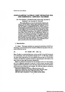
gene sets s = 1 and 2 are active and gene set 0 is inactive. Cells in white represent inactive samples (such as sample cluster 0 in gene set 2). The remaining cells with matching colors in same column form sample clusters. Distinct colors indicate ? distinct θkg . For example, Gene set 2 has three sample clusters. Sample cluster 0 is inactive including samples {S2, S4, S7, S8}. Clusters 1 and 2 are active, including {S3, S5, S9} and {S1, S6}, respectively. Within each gene set, the colors corresponding to an active sample cluster vary across columns, because gene sets are defined by matching partitions cs across all columns g with wg = s, rather than by matching means θig . This is a key characteristic of the proposed model. In contrast, most existing clustering approaches would assume that the row clusters are represented by the same color across columns, e.g. sample cluster 1 for gene set 2 would all have green color under most existing clustering methods. 2 2 2 , τ1g , and τ2g . We use an inverse We complete the model with priors for σg2 , τ0g 2 gamma distribution σg ∼ IG(ag , bg ) independently across g . Similarly, we 2 consider an inverse gamma distribution τ`g ∼ IG(a`g , b`g ) independently across g for ` = 0, 1, 2. The hierarchical model is summarized in Figure 2. 3.
Posterior Inference
Let θ denote the vector of all θig parameters, and similarly for τ and σ 2 . The joint distribution of data and parameters is summarized as p(Y , w, c, θ, σ 2 , τ 2 ) = p(w) p(c | w) p(θ | w, c, τ 2 ) p(Y | θ, σ 2 ) p(σ 2 ) p(τ 2 ). We use Markov chain Monte Carlo (MCMC) simulation to implement pos? 2 2 terior inference. We iteratively update (i) θig (or θkg ); (ii) σg2 ; (iii) τ0g , τ1g and 2 τ2g ; (iv) cs ; and (v) w. Each update is implemented by a transition probability conditional on the currently imputed values of all other parameters. When updating w and cs , we sequentially remove a gene or a sample from w and cs , respectively, and draw a new cluster label from the full conditional posterior distributions, marginalized with respect to θ. Also, we make use of a pseudo prior mechanism (Carlin and Chib, 1995) to construct a proposal for cs when we implement a transition probability for wg . We introduce a set of auxiliary variables e cg , g = 1, . . . , G with e cg = (e cgi , i = 1, . . . , N ). Think of e cg as a potential sample partition that could be used under a singleton gene set {g}. 2 2 ) for the auxiliary variables We define a model augmentation p(e cg | y g , τ0g , τ1g e cg to be identical to what the posterior on cs would be for a singleton gene set {g}. We then use e cg in the construction of a Metropolis-Hastings proposal for wg . Specifically, when considering wg = S + 1, that is, when proposing a new singleton gene set, we make a joint proposal (wg = S + 1, cS+1 = e cg ). In other words, the proposal distribution for the sample partition under the new gene set is deterministic by copying the currently imputed value e cg . More technical details of the posterior MCMC are listed in the supplementary materials. 7
Our model provides full posterior inference on the gene sets and their corresponding sample clusters. Summarizing this posterior distribution starts with the report of a point estimate for the random partition. We face the practical problem of summarizing a distribution over partitions. Medvedovic and Sivaganesan (2002) and Medvedovic et al. (2004) attacked this problem by reporting posterior probabilities that any two genes are grouped together. Dahl (2006) went a step further and introduced a method to obtain a point estimate of the random clusters based on least-square distance from the matrix of posterior pairwise co-clustering probabilities under a Dirichlet process mixture model. Both methods start with an association matrix, Dw , of dimension G × G whose 0 (g, g 0 ) element, dw g,g 0 = I(wg = wg 0 ) is an indicator of whether genes g and g are grouped together. Then they compute a matrix Q of posterior pairwise coclustering probabilities as the mean of dw g,g 0 across the posterior samples. To take account of the inactive gene set in our model, we let dg,g0 = 0 for all g 0 if wg = 0. Following Dahl (2006), we use the least-squares summary wLS defined as wLS = arg min ||Dw − Q||2 . w By definition, wLS minimizes the sum of the squared deviation of its association matrix from the matrix of the posterior pairwise co-clustering probabilities. The estimate wLS defines the number and configuration of the gene sets. Conditional on each gene set implied by wLS , we extract the MCMC samples of c corresponding to the gene set and compute the least-squares estimate cLS s , s = 1, . . . , S LS as the sample clusters. 4.
Simulation
We examined the proposed model through a simulation study comparing model estimates with the simulation truth and with inference under three alternative methods, the plaid model (Lazzeroni and Owen, 2002; Turner et al., 2005), the sparse hierarchical clustering (Witten and Tibshirani, 2010), and the DCIM model (Freudenberg et al., 2010). We simulated 20 genes (G = 20) with 120 samples (N = 120). We assumed three gene sets including an inactive gene set, (s = 0, 1, 2), where gene set 1 has 8 genes and gene set 2 has 7 genes. Gene set 1 partitions the samples into four sample clusters including an inactive sample cluster (k = 0, . . . , 3). We generated sample cluster labels c1i for gene set 1, assuming that a sample belongs to one of the four sample clusters with equal probability. Similarly, gene set 2 has three sample clusters including an inactive sample cluster (k = 0, . . . , 2). Again, we generated c2i assuming that a sample has equal probability of belonging to one of the three sample clusters. For the inactive gene set 0, we did not generate sample clusters, according to the definition of the inactive gene set. To make the simulation setup more challenging and realistic, we allowed genes 6–8 to be in both gene sets 1 and 2. Specifically, we let genes 1–8 belong to gene 8
set 1 and genes 6–12 belong to gene set 2. See the supplementary materials for ? ? the remaining details of how θkg and θig are generated. One realization of θkg for gene sets 1 and 2 is listed in Table 1. For the three common genes, genes 6–8, a sample follows a cluster membership of gene set 1 or gene set 2 with ? ? equal probability, and the corresponding θig is either θkg in Table 1a or θkg in 2 Table 1b. Finally, we generated yig ∼ N(θig , σg ) where σg = 0.3. Figure 3 illustrates the heatmaps of yig for each of the three true gene sets (s = 0, 1, 2). After rearranging genes and rearranging samples within each gene set according to the simulation truth, we observed clear local clustering patterns in the data. For the three common genes, samples are rearranged according to the sample cluster membership of true gene set 1. For better presentation, in the figure, yig were rescaled to zero mean and unit variance in each column. In gene sets 1 and 2 , the inactive samples are displayed in the first block of rows and show large variability in the color-coded expression levels. The active samples show more uniform colors within each sample cluster. Since for genes 6–8 the sample clustering arises as a mixture of clustering under gene sets 1 and 2, their expression levels show larger variability even in active sample clusters. In gene set 0, samples do not cluster and the corresponding gene expression levels show large variability. Figure 4 shows the estimated clustering results under hierarchical clustering, implemented in R using the function heatmap.2(). The global clustering of genes (samples) is based on all samples (genes). Therefore, hierarchical clustering did not provide true local clustering patterns in the data. We implemented posterior simulation for inference under the proposed NoBLoC model. We used the result from hierarchical clustering to initialize w: We cut the dendrogram of the hierarchical clustering of genes to have 12 gene clusters including 5 singleton clusters. For the initialization we combined the five singleton clusters to define an inactive gene set, s = 0. We fixed µ0g = µ1g = µ2g at the sample median, med(yig , i = 1, . . . , N ), π0 = 0.6 and π1 = 0.8. We specified the hyperparameters alg , blg , ag and bg , by fixing the mean and 2 variance of the inverse gamma priors for σg2 and τlg . Specifically, we matched 2 2 2 2 ) = E(τ0g ) = E(τ1g ) = E(τ2g ) with the sample variance of yig and set Var(τ0g 2 2 2 2 Var(τ1g ) = Var(τ2g ) = 0.4. Also we centered p(σg ) by setting E(σg ) equal to the simulation truth and Var(σg2 ) = 0.4. We then implemented posterior inference using MCMC posterior simulation. We ran the MCMC simulation over 20,000 iterations, discarding the first 5,000 iterations as burn-in. The least-squares summary of the posterior on w is wLS = (1, 1, 1, 1, 1, 1, 1, 1, 2, 2, 2, 2, 0, 0, 0, 0, 0, 0, 0, 0, 0). The estimated clustering wLS indicated that genes 1–8 and 9–12 occurred in two different gene sets, while the remaining genes in the inactive gene set. Recall that under the simulation truth, for genes 6 – 8 samples may follow either the sample clustering of true gene set s = 1 or s = 2. Conditional on wLS , we computed the least-squares estimates of sample clus9
ters for the two gene sets, cLS s , s = 1, 2 and compared the estimated cluster membership to the truth, shown in Table 2. Table 2a shows that there are 11 estimated sample clusters for gene set 1, with clusters (columns in Table 2a) {0, 1, 2, 4} dominating and largely overlapping with the four true sample clusters of true gene set 1 (including the inactive one). There were some additional small sample clusters, with labels {3, 5–11}. Those small sample clusters accommodate the mixture clustering of true gene sets 1 and 2 with respect to genes 6–8 in gene set 1 of wLS . The reported inference is a reasonable approximation of the simulation truth within the assumed analysis model. Table 2b shows that posterior inference identifies the true cluster membership of true gene set 2 well. Figure 5 shows the heatmaps for each gene set of wLS . Comparing with the simulation truth in Figure 3, the only discrepancy was the additional sample clusters under gene set 1. Those were samples whose simulated cluster membership was determined by a mixture of the partitions c1 and c2 . As comparison, we carried out inference for the same simulated data using three alternative methods, including the plaid model, the sparse hierarchical clustering and the DCIM model. The three methods are implemented in the R packages, biclust, sparcl and gimmR, respectively. See the supplementary materials for figures with corresponding heatmaps. Here we only summarized the main features of the inference under the three alternative approaches. The plaid model identified only one bicluster of 22 samples with three genes {6, 10, 11}. Most of the samples were in true sample cluster 2 of true gene set 2. The sparse hierarchical clustering produced two sets of sample clusters. The first set was obtained through a direct implementation of the model in Witten and Tibshirani (2010), and the second set of clusters was obtained after removing the effects found in the first clustering from the data, as suggested by the authors. Each of the partitions is based on its own chosen subset of genes. The first clustering chose 7 genes, {3, 6, 7, 8, 9, 10, 12}, and the second clustering chose 9 genes, {1, 3, 5, 8, 13, 14, 15, 17, 20}. The genes chosen by the first clustering largely overlapped with the genes in true gene set 2. We cut the resulting dendrogram to form three sample clusters. We chose the number of clusters to favor a match with the simulation truth that included K = 3 sample clusters under true gene set 2. Similarly, the genes chosen by the second clustering were mostly in true gene set 1 and in the true inactive gene set. We cut the resulting dendrogram and formed four sample clusters. The sample cluster memberships of the first and second clusterings were compared to true cluster memberships of gene sets 2 and 1, respectively. Table 3 summarizes the comparison. The sample partitions from the sparse hierarchical clustering did not match well with the true sample partitions, perhaps because the sparse hierarchical clustering forces all the samples to be assigned to a cluster. The sparse hierarchical clustering may also suffer from the inclusion of inactive genes and the embedded structure in the true gene sets. The DCIM model summarized the posterior inference as two sets of global hierarchical clusters, one for genes and the other for samples. The DCIM model 10
forms contexts of samples in which genes are similarly clustered. How the DCIM model forms contexts is similar to the formation of gene sets in our model. We therefore transposed the data matrix before applying the DCIM model and reported the resulting clustering of genes and the global partition of samples. We first cut the dendrogram for genes to form three gene sets. We then considered the dendrogram for samples corresponding to the global sample clusters, separately for each of the gene sets to form gene-set-specific sample partitions. The three gene sets were identical to the gene sets characterized by wLS under the NoB-LoC model. Table 4 illustrates the comparison of the sample cluster memberships for the first two gene sets. In Table 4a we see that inference under the DCIM model does not entirely separate inactive samples or capture the embedded structure. Table 4b exhibits the misclassification of many samples. We cut the dendrogram for gene set 3, the true inactive gene set, to form five sample clusters. This number was arbitrarily chosen after inspection of the dendrogram. The resulting sample clusters were noisy because gene set 3 was truly inactive in the simulation truth (shown in Figure 3 in the supplementary materials). In contrast, the NoB-LoC model correctly identified this gene set as inactive and did not attempt to partition the samples. Overall, for this simulation study, the NoB-LoC method did well in capturing clustering patterns in a two-way matrix, compared to the other three methods.
5.
RPPA Data
We analyzed data from an experiment using reverse phase protein arrays (RPPA). RPPA allows simultaneous quantification of protein expression levels in a large number of biological samples (Tibes et al., 2006). The data set included the expression levels of G = 56 proteins that were selected from two cell signaling pathways for N = 256 samples from breast cancer patients. The heatmap of the data set is shown in Figure 6 along with the dendrograms from hierarchical clustering. Hierarchical clustering identified four major groups of proteins based on all the samples and, vice versa, it found five major clusters of samples based on data from all the proteins. To fit the NoB-LoC model, we initialized w based on the results from hierarchical clustering. We cut the hierarchical clustering tree of proteins at a level that produced 13 protein clusters and combined all singleton protein clusters into the inactive protein set. We matched µ0g = µ1g = µ2g with the sample median, med(yig , i = 1, . . . , N ) and fixed π0 = 0.86 and π1 = 0.5. To set the hyperpa2 2 2 ) = E(τ2g ) to match rameters a`g , b`g , ag and bg , we chose values E(τ0g ) = E(τ1g 2 2 2 ) = 1. the sample variance of the yig and fixed Var(τ0g ) = Var(τ1g ) = Var(τ2g 2 We set E(σg ) equal to the sample variance of yig after trimming 5% from each tail and fixed Var(σg2 ) = 5. We implemented inference using MCMC posterior simulation by sampling over all the complete conditionals for 35,000 iterations, discarding the first 5,000 iterations as burn-in. 11
We computed the least-squares estimates of protein sets and the corresponding sample clusters, wLS and cLS s . The NoB-LoC model identified four protein sets, each of which partitioned samples differently. The protein sets are shown in Figure 7. In the figure, each panel shows the composition of protein sets and the corresponding sample clustering, with the inactive sample clusters on the first block of rows for each active protein set. The inferred sample clusters were clearly visible as well defined blocks of color-coded protein expression. The RPPA data set included three important biomarker proteins: ER, PR and HER2 ( 54, 55 and 56 in the figures). The biomarker proteins ER and HER2 belonged to protein set 3, and PR belonged to protein set 1 in wLS . The cancer subtypes HR+, HER2+ and TN were defined based on these three biomarker proteins. For samples with subtype HR+, either ER or PR is over-expressed, but HER2 is under-expressed. For samples with subtype HER2+, HER2 is overexpressed regardless of the expression of ER or PR. For samples with subtype TN, all the three biomarker proteins are under-expressed. In comparing the local sample clusters with the clinical subtypes of the samples, we found that protein sets 1, 2, and 3 roughly separated samples with subtype HR+ from samples with subtypes HER2+ and TN. This agrees with the prior knowledge that subtype HR+ has very different characteristics from subtypes HER2+ and TN. However, overall there was little overlap between the local clusters identified by the NoB-LoC method and the clinical definition. This is no surprise, as the clinical definition of subtypes has not yielded clear and successful prognosis, suggesting poor understanding and perhaps inadequate knowledge of different subtypes of breast cancer. For comparison we applied the plaid model, the sparse hierarchical clustering and the DCIM model to the same data set. First, the plaid model identified two biclusters. One consisted of proteins {4, 5, 18} with 27 samples, and the other had two proteins {4, 5} with 43 samples. The samples in the two biclusters did not naturally correspond to any of the clinical subtypes. We also applied the sparse hierarchical clustering approach. It chose all the proteins except protein 18 for its first clustering and all the proteins for the second clustering. The dendrograms were cut to form three sample clusters to favor a possible match with the three clinical subtypes. A comparison of the sample partitions with the three cancer subtypes found no natural match. Finally, we applied the DCIM model to the data. We cut the dendrogram of the protein clustering in the DCIM model to form four protein sets, and we cut the dendrogram of the global sample clustering in the DCIM model to form three sample clusters. Again, we chose the cut into three sample clusters to favor a possible match with the three clinical subtypes. However, the resulting sample partition does not show any natural match with the three clinical types. Note that the first estimated protein set included all the proteins in protein sets 1, 2 and 3 implied by wLS under the NoB-LoC model, except for proteins 54 and 55. The NoB-LoC model assigned those proteins into three separate protein sets and allowed the three protein sets to partition samples differently. In contrast, 12
the DCIM model inferred one common sample partition for those proteins.
6.
Mass Cytometry Data
We analyzed the mass cytometry (Bendall et al., 2011) data presented in Qiu et al. (2011). Mass cytometry is a new single-cell technology that measures protein biomarkers simultaneously in individual cells using a mass cytometer (CyTOFTM ). The resulting multidimensional measurements of individual cells allow researchers to study cells in heterogeneous populations such as immunophenotyping blood markers in the diagnosis of leukemia subtypes (Ornatsky et al., 2010). The data set was a subset of data in Bendall et al. (2011) randomly chosen by our collaborator, which reported measurements for 31 protein biomarkers (columns) and 200 cells from human bone marrow (rows). Among the 31 proteins, 13 were surface markers, numbered from 1 through 13 and the remaining 18 proteins were unstimulated functional proteins, numbered from 14 through 31. On the basis of the entire data, Qiu et al. (2011) defined 6 different cell types based on all the 13 surface protein biomarkers. The clustering result in Qiu et al. (2011) included 43, 34, 27, 26, 51, and 19 cells in the 6 cell types for our data set. For simplicity, we denote the six cell types as {A, B, C, D, E, F}. Figure 8 shows a heatmap of the data with dendrograms from hierarchical clustering. Based on data from all the cells, hierarchical clustering suggested four major protein clusters, and based on data from all the proteins we recognized five cell clusters. The nature of the data makes the proposed NoB-LoC model ideal for inference about cell types. The investigators expect that subsets of markers define different sets of cell types. In other words, for different subsets of markers (columns) we should be able to cluster a subset of the cells (rows) into coherent types, leaving the remaining cells as not classified with respect to these markers. To fit the proposed NoB-LoC model we started with initial values for the MCMC posterior simulation. We initialized w based on the results from the hierarchical clustering of proteins. We cut the hierarchical clustering tree of proteins to obtain 12 protein clusters, including 7 singleton clusters. We used the result for the initial w, combining the singleton clusters into one inactive protein set. We fixed µ0g = µ1g = µ2g by matching them with the sample median, med(yig , i = 1, . . . , N ), and set π0 = 0.77 and π1 = 0.5. To set 2 2 2 ) = E(τ1g ) = E(τ2g ) with hyperparameters ag , bg a`g and b`g , we matched E(τ0g 2 2 2 the sample variance of the yig , and fixed Var(τ0g ) = Var(τ1g ) = Var(τ2g ) = 1. We set E(σg2 ) to match the variance of yig after trimming 5% from each tail, and fixed Var(σg2 ) = 2. We implemented posterior inference using MCMC posterior simulations for the proposed model. We ran the MCMC simulation by iterating over all complete conditionals for 20,000 iterations, discarding the first 5,000 iterations as burn-in. 13
We computed the least-squares estimates of protein sets and the corresponding cell clusters, wLS and cLS s . The NoB-LoC model identified two active protein sets and one inactive protein set. Protein set 1 included 28 proteins and protein set 2 included 2 proteins. Protein set 0, the inactive one, only had one protein. The heatmaps of the three protein sets are shown in Figure 9. The comparison of cell clustering with the predefined 6 cell types is given in Table 5. Overall, the cell clustering of protein set 1 shown in (a) matches well with the predefined 6 cell types. Exceptions are cell clusters 2 and 6 in cLS 1 , which are both dominated by cells with predefined type A. This mismatch may indicate the existence of an embedded structure within cell type A. As shown in Figure 9, protein set 2 in wLS includes proteins 7 and 14. This indicates that those two proteins do not provide information related to the 6 predefined cell types, which was also noted by our collaborator in the previous analysis in Qiu et al. (2011). However, the two proteins together may characterize an alternative clustering of cells. Further experimental validation is needed. For comparison, we report inference for the same data under the plaid model, the sparse hierarchical clustering and the DCIM. The plaid model identified four biclusters. Bicluster 1 included three proteins, {2, 6, 13} with 36 cells. Bicluster 2 included the same three proteins as in bicluster 1 but with 11 cells. Bicluster 3 included three proteins {4, 9, 25} with 27 cells. Finally, bicluster 4 included two proteins, {5, 13} with 23 cells. Table 6 compares the biclusters with the predefined cell types. The plaid model did not have biclusters of cells with types C and F which are types having relatively fewer cells in the data. The sparse hierarchical clustering chose 21 proteins for the first clustering and 22 proteins for the second clustering. The two clusterings chose 18 common proteins. Each of the dendrograms was cut to form six cell clusters to favor a possible match with the pre-defined cell types. Table 7 compares the cluster memberships to the pre-defined cell types. We found no obvious match. For example, in Table 7a cells with cell types D and E were grouped together in cluster 1 and approximately half of cells with cell types A and B were grouped together in cluster 4. Finally, we applied the DCIM model to the same data. We cut the dendrogram of the protein clustering to form two protein sets, and similarly we cut the dendrogram of the global cell clustering to form six cell clusters. Since the cell clusters were based on the global cell clustering, they were common for the two protein sets. We again compared the cell cluster memberships to the six pre-defined cell types. As shown in Table 8, with the six clusters of the DCIM model, pre-defined cell types D and E were grouped together in cluster 1. 7.
Conclusions
The proposed model extracts local clusters from a data matrix. The model characterizes local clustering by assuming that sample partitions are nested with gene sets. We achieve robust estimates of local clustering patterns by explicitly 14
excluding noisy genes (proteins) and samples from clustering. Through the simulation study and the analysis of the two data sets, we have showed that the proposed model provides potentially useful insights. We use a zero-enriched P´ olya Urn scheme to model random partitions of genes and samples. If desired, any alternative random partition model could be substituted without substantially changing the approach. Alternative models could be used to represent different prior judgement on the number and relative sizes of the clusters. The model could be adequately adjusted according to the purpose of data analysis. The currently used partition of genes could be relaxed to a family of subsets, with possible overlap. This would reflects that many genes can feature in multiple biologic processes. The lack of such overlap is a limitation of the proposed model. Another direction of possible extensions is the sampling model. The assumed normal sampling model could be replaced by essentially arbitrary other models without any change in the underlying probability models on the random partitions. Supplementary Materials Supplementary materials are available under the Paper Information link at the JRSS-B website http://www.wiley.com/bw/journal.asp?ref=1369-7412&site=1. Acknowledgement The authors thank Peng Qui for providing the mass cytometry data and helpful insights on the data. Yuan Ji and Peter M¨ uller’s research is partially supported by NIH R01 CA132897. References Belacel, N., Wang, Q. C., and Cuperlovic-Culf, M. (2006). Clustering methods for microarray gene expression data. OMICS: A Journal of Integrative Biology 10, 4, 507–531. Bendall, S. C., Simonds, E. F., Qiu, P., ad D. Amir, E., Krutzik, P. O., Finck, R., Bruggner, R. V., Melamed, R., Ornatsky, O. I., Balderas, R. S., Plevritis, S. K., Sachs, K., Pe’er, D., Tanner, S. D., and Nolan, G. P. (2011). Single cell mass cytometry of differential immune and drug responses across the human hematopoietic continuum. Science 332, 6030, 687–696. Carlin, B. P. and Chib, S. (1995). Bayesian model choice via Markov chain Monte Carlo methods. Journal of the Royal Statistical Society, Series B: Methodological 57, 473–484. 15
Cheng, Y. and Church, G. M. (2000). Biclustering of expression data. Proceedings of the Eight International Conference on Intelligent Systems for Molecular Biology (ISBM) 8, 93–103. Dahl, D. B. (2006). Model-Based Clustering for Expression Data via a Dirichlet Process Mixture Model. In M. Vannucci, K.-A. Do, and P. M¨ uller, eds., Bayesian Inference for Gene Expression and Proteomics. Cambridge University Press. Dunson, D. B. (2009). Nonparamaetric Bayes local partition models for random effects. Biometrika 96, 2, 249–262. Fraley, C. and Raftery, A. E. (2002). Model-based clustering, discriminant analysis, and density estimation. Journal of the American Statistical Association 97, 458, 611–631. Freudenberg, J. M., Sivaganesan, S., Wagner, M., and Medvedovic, M. (2010). A semi-parametric bayesian model for unsupervised differential co-expression analysis. BMC Bioinformatics 11, 234. Jiang, D., Tang, C., and Zhang, A. (2004). Clustering analysis for gene expression data: a survey. IEEE Transactions on Knowledge and Data Engineering 16, 1370–1386. Lazzeroni, L. and Owen, A. (2002). Paid Models for Gene Expression Data. Statistica Sinica 12, 61–86. Medvedovic, M. and Sivaganesan, S. (2002). Bayesian infinite mixture model based clustering of gene expression profiles. Bioinformatics 18, 9, 1194–206. Medvedovic, M., Yeung, K., and Bumgarner, R. (2004). Bayesian mixture model based clustering of replicated microarray data. Bioinformatics 22, 8, 1222–32. Meeds, E. and Roweis, S. (2007). Nonparametric bayesian biclustering. Tech. rep., Department of Computer Science, University of Toronto. M¨ uller, P., Quintana, F. A., and Rosner, G. L. (2011). A product partition model with regression on covariates. Journal of Computational and Graphical Statistics 20, 1, 260–278. Ornatsky, O., Bandura, D., Baranov, V., Nitz, M., Winnik, M., and Tanner, S. (2010). Highly multiparametric analysis by mass cytometry. Journal of Immunological Methods 361, 1–20. Petrone, S., Guindani, M., and Gelfand, A. E. (2009). Hybrid Dirichlet mixture models for functional data. Journal of the Royal Statistical Society, Series B: Statistical Methodology 71, 4, 755–782. 16
Qiu, P., Simonds, E. F., Bendall, S. C., Jr., K. D. G., Bruggner, R. V., Linderman, M. D., Sachs, K., Nolan, G. P., and Plevritis, S. K. (2011). Extracting a cellular hierarchy from high-dimensional cytometry data with spade. Nature Biotechnology 29, 10, 886–891. Quintana, F. A. (2006). A predictive view of Bayesian clustering. Journal of Statistical Planning and Inference 136, 8, 2407–2429. Sivaganesan, S., Laud, P. W., and M¨ uller, P. (2011). A Bayesian subgroup analysis with a zero-enriched Polya Urn scheme. Statistics in Medicine , 4, 312–23. Tibes, R., Qiu, Y., Lu, Y., Hennessy, B., Andreeff, M., Mills, G. B., , and Kornblau, S. M. (2006). Reverse phase protein array: validation of a novel proteomic technology and utility for analysis of primary leukemia specimens and hematopoietic stem cells. Molecular Cancer Therapeutics 5, 2512–2521. Turner, H., Bailey, T., and Krzanowski, W. (2005). Improved biclustering of microarray data demonstrated through systematic performance tests. Computational Statistics & Data Analysis 48, 235–254. Witten, D. M. and Tibshirani, R. (2010). A framework for feature selection in clustering. Journal of the American Statistical Association 105, 490, 713–726.
17
Gene set 1
Gene set 0 G5
G1
Gene set 2
G3
G2
S1
S1
S2
S2
S4
S4
S3
S2
S7
S4
S3
S8
S5
S6
S3
S6
S5
S5
S7
S7
S9
S8
S8
S1
S9
S9
S6
G4
G6
Sample cluster 0
Sample cluster 1
Sample cluster 2
Fig. 1. An illustration of the NoB-LoC model. Partition of genes (columns) and nested partition of samples (rows).
18
g =1, …, G genes π
0
α
s =1, …, S gene sets
Gene set configuration
€
€
Sample clustering € configuration
€csi
j =1, …, K s samples clusters €
€
µ2g
2 τ0g
µ0g
€
θ jg* € 2 τ2g
µ1g
€
€
θ ig €
π1
M
wg
€
€
τ1g2
σg2
€ €
€yig
i =1, …, N samples
Fig. 2. Graphical representation€of the NoB-LoC model.
19
Table 1. Locations of sample clusters for the simulated data. (a) Locations for gene set 1
cluster 1 cluster 2 cluster 3
gene 1 -0.87 -0.50 0.29
gene 2 0.73 -0.35 0.36
gene 3 -0.26 -0.73 0.47
gene 4 -0.66 0.48 -0.52
gene 5 0.41 -0.32 -0.88
gene 6 -0.37 0.40 -0.05
gene 7 -0.47 -0.99 0.80
gene 8 -0.01 0.52 0.96
(b) Locations for gene set 2
cluster 1 cluster 2
gene 6 -0.67 0.89
gene 7 0.52 0.10
gene 8 -0.38 -0.95
gene 9 0.43 -0.84
20
gene 10 -0.93 0.58
gene 11 -0.49 0.29
gene 12 0.44 -0.61
Color Key and Histogram 80
1
2
80 40 0 −2
0
1
2
Column Z−Score gene set 2 Color Key and Histogram
−2
0
1
2
21
4
8 15
13
6
1
Fig. 3. Heatmaps of the three true gene sets in the simulated data. The samples are rearranged according to the simulation truth in gene sets 1 and 2. For genes 6–8 samples are rearranged according to the sample cluster membership of true gene set 1. White horizontal lines show division of clusters. The first block of top rows for each gene set represents the inactive samples for that gene set. The remaining row blocks are active sample clusters.
3
gene set 3 Column Z−Score
2
Count
40 80 0
0
and Histogram
Count
Count
−2
Column Z−Score gene 1 Colorset Key
80
12 34 56 879 1011 131214 1516 1718 1920 222123 2425 2627 292830 323133 3435 3637 3839 414042 4344 4546 484749 515052 5354 5556 5758 605961 6263 6465 676668 6970 7172 747375 777678 7980 8182 8384 868587 8889 9091 939294 969597 9899 100 101 102 103 104 105 106 107 108 109 110 111 112 113 114 115 116 117 118 119 120
40
12 34 56 879 111012 1314 1516 1718 201921 2223 2425 272628 302931 3233 3435 3637 393840 4142 4344 464547 4849 5051 535254 565557 5859 6061 6263 656466 6768 6970 727173 757476 7778 7980 8182 848385 8687 8889 919092 949395 9697 9899 100 101 102 103 104 105 106 107 108 109 110 111 112 113 114 115 116 117 118 119 120
Color ColorKeys Key and Histogram
7
9 9 10 11 11 12 12 10
11 22 33 44 55 6 66 7 77 88 8
12 435 67 9810 1112 1314 1516 181719 2021 2223 252426 282729 3031 3233 3435 373638 3940 4142 444345 474648 4950 5152 5354 565557 5859 6061 636264 6566 6768 706971 737274 7576 7778 7980 828183 8485 8687 898890 929193 9495 9697 9899 100 101 102 103 104 105 106 107 108 109 110 111 112 113 114 115 116 117 118 119 120
gene set 0
14
0 1 2
0
−2
gene set Colu2 mn Z−Score
13 14 15 15 16 16 17 17 18 18 19 19 20 20
0 1 2
14
−2
gene set 1 Column Z−Score
13
0 1 2
0
0
−2
Column Z−Score
40
Count
80
Color Key and Histogram
40
Count
80 40 0
Count
Color Key and Histogram
250 100 0
Count
Color Key and Histogram
−2
0
1
2
Column Z−Score
6
10
8
11
7
3
1
2
15
5
13
18
19
14
16
20
4
17
9
12
20 77 60 74 85 88 48 2 63 26 96 44 81 117 41 114 3 79 86 54 107 65 56 66 72 87 102 29 14 68 17 8 120 11 100 91 22 118 109 10 34 99 67 30 21 25 111 110 38 45 51 16 24 104 33 76 32 7 42 13 113 61 64 4 73 43 98 12 53 112 1 89 55 69 19 58 94 119 46 27 83 23 15 50 35 116 95 80 47 106 78 5 28 115 9 70 103 39 75 92 37 36 97 93 101 40 108 52 49 62 6 82 71 31 84 59 105 90 18 57
Fig. 4. A Heatmap of the simulated data. Dendrograms are estimated using hierarchical clustering.
22
Table 2. Comparison of the estimated clustering membership by the NoB-LoC model for the simulated data. The least-squares sample clusterings, cLS and cLS are com1 2 pared to the clusterings of true gene sets 1 and 2, respectively. (a) Gene set 1 of NoB-LoC T RU E
c k k k k
=0 =1 =2 =3
0 19 1 1 0
1 1 0 0 23
2 1 0 22 0
3 1 0 0 6
4 0 21 0 0
cLS 1 5 0 4 0 0
6 3 0 5 0
7 2 0 0 0
(b) Gene set 2 of NoB-Loc T RU E
c k=0 k=1 k=2
cLS 2 1 4 38 0
0 31 1 0
23
2 1 0 45
8 2 0 0 0
9 2 0 0 4
10 1 0 0 0
11 1 0 0 0
Color Key and Histogram 80
0 1 2
12 435 67 89 1011 131214 1516 1718 201921 232224 2526 2728 2930 323133 3435 3637 393840 424143 4445 4647 4849 515052 5354 5556 585759 616062 6364 6566 6768 706971 7273 7475 777678 7980 8182 848385 878688 8990 9192 9394 969597 9899 100101 103102104 106105107 108109 110111 112113 115114116 117118 119120
Color ColorKeys Key and Histogram
−2
Count
1
2
0
20
40
and Histogram
−2 −1
0
1
2
Column ColorZ−Score Key2 gene set 80
and Histogram
−2
0
1
2
24
4
10
16
15
14
13
9
1
Fig. 5. Heatmaps of three identified gene sets for the simulated data using the NoB-LoC model. The samples are rearranged according to the estimated cluster membership for gene sets 1 and 2. White horizontal lines show division of clusters. The first block of top rows for each active gene set represents the inactive samples for that gene set. The remaining row blocks are active sample clusters.
3
Column Z−Score gene set 3
2
13 14 15 15 16 16 17 17 18 18 19 19 20 20
0
Column Z−Score gene 1 Colorset Key
Count
Count
0
40 80
12 34 56 879 111012 1314 1516 1718 201921 2223 2425 272628 302931 3233 3435 3637 393840 4142 4344 464547 4849 5051 535254 565557 5859 6061 6263 656466 6768 6970 727173 757476 7778 7980 8182 848385 8687 8889 919092 949395 9697 9899 100 101 102 103 104 105 106 107 108 109 110 111 112 113 114 115 116 117 118 119 120
14
12
11
9 10 11 12 9
10
1 1 2 2 3 3 4 4 5 5 6 6 7 7 8 8
12 435 67 89 1011 131214 1516 1718 201921 232224 2526 2728 2930 323133 3435 3637 393840 4142 4344 464547 494850 5152 5354 5556 585759 6061 6263 656466 686769 7071 7273 7475 777678 7980 8182 848385 878688 8990 9192 9394 969597 9899 100 101 102 103 104 105 106 107 108 109 110 111 112 113 114 115 116 117 118 119 120
gene set 0
40
−2
0
−2 −1 0 1 2
gene set 1 Column Z−Score gene Columnset Z−Score2
13
0 1 2
0
0
−2
Column Z−Score
40
Count
40
Color Key and Histogram
20
Count
80 40 0
Count
Color Key and Histogram
Table 3. Comparison of the estimated sample cluster membership in the sparse hierarchical clustering for the simulated data. The cluster memberships of the first and second clustering are compared to those of the true gene sets 2 and 1, respectively. The clusters are obtained by cutting the dendrograms. (a) First clustering cT RU E k=0 k=1 k=2
Estimated clusters 1 2 3 15 10 11 1 0 38 32 13 0
(b) Second clustering cT RU E k=0 k=1 k=2 k=3
Estimated clusters 1 2 3 4 12 0 15 6 0 0 6 20 0 4 18 6 6 19 8 0
25
Table 4. Comparison of sample cluster membership from the DCIM model for the simulated data. The sample cluster memberships of gene sets 1 and 2 from the DCIM model are compared to those of true gene set 1 and 2, respectively. The clusters are obtained by cutting the dendrograms. (a) Gene set 1 of DCIM
cT RU E k=0 k=1 k=2 k=3
Estimated clusters 1 2 3 4 4 6 8 15 0 0 0 12 0 0 15 0 0 19 0 0
(a) Gene set 2 of DCIM
cT RU E k=0 k=1 k=2
Estimated clusters 1 2 3 9 10 17 9 5 25 30 10 5
26
2000 0
Count
Color Key and Histogram
−4
0
2
4
Column Z−Score
6 45 50 14 23 29 49 9 3 28 17 56 55 2 11 12 20 42 25 52 27 26 13 7 8 30 54 24 31 39 19 53 10 16 44 46 1 35 32 36 41 51 34 22 38 40 43 37 33 48 21 15 47 4 5 18
215 164 220 173 44 89 141 196 116 208 198 179 194 207 112 167 106 82 114 120 227 28 243 213 171 236 200 184 70 231 203 181 237 139 224 8 145 189 59 166 172 214 80 107 117 26 209 183 229 178 187 170 91 174 2 240 197 249 253 250 221 96 242 21 202 113 225 248 255 54 36 67 72 25 222 251 159 158 142 148 43 239 51 165 20 190 134 109 94 135 48 143 30 132 4 18 217 121 124 252 152 219 68 127 211 238 218 169 140 182 177 193 100 210 201 246 254 168 235 16 180 161 83 38 9 176 77 101 247 204 212 188 195 163 11 103 234 58 136 60 119 37 15 123 69 92 191 108 53 102 137 150 131 22 24 79 71 111 64 63 192 62 115 57 17 65 205 74 46 230 81 185 88 118 78 151 133 99 216 154 245 155 90 122 12 146 5 144 33 66 3 35 228 32 19 241 156 41 256 125 244 206 29 98 129 104 56 95 14 27 199 93 31 6 75 47 157 50 55 175 162 86 76 40 7 149 23 49 160 34 84 39 186 128 130 110 42 45 52 138 126 223 232 1 97 105 61 87 233 13 226 85 73 10 153 147
Fig. 6. A heatmap of the RPPA data set. Dendrograms are estimated using hierarchical clustering.
27
150
Count
50 0
Color Keys 500
Count
200 0
800
−4 −2
2
4
ps2
1000
Color Key and Histogram
400
Count
ps3
0
Column Z−Score
0
800
Count
400 0
1 43265 and Histogram 98710 111142356 121290781 22345 23289067 312 33335467 44301892 44435 6 4554490178 523 55556478 −3 −1 1 3 66619032 Column Z−Score 66457 776601289 734 7775689 Color Key 88820143 888567 and Histogram 99991230 45 99918670 1110002354 1100678 109 1112340 156 11129780 11111222224365 127890 11113333425 113367 −3 −1 1 2 3 1114340892 1114445376 Column Z−Score 111445890 11111555554236 Color Key 1578 111165669023 and Histogram 111166664587 1167790 172 111177775634 1118780892 118834 111188887569 11199902 193 11199967458 2212009013 222000456 7 2222211100089 −2 0 2 2134 22211178569 222223014 Column Z−Score 22567 223890 22331 222333465 2223348970 22224444315 2244678 22455901 225534 256
ps1
400
Count
Color Key and Histogram
Color Key
0
21 54376 10981211 131514 1817162019 2322212524 2827263029 313332 343635 3938374140 4443424645 4948475150 5453525655 575958 606261 6564636766 7069687271 7574737776 788079 818382 8685848887 9190899392 9695949897 10110099103102 104106105 107109108 112111110114113 117116115119118 122121120124123 127126125129128 130132131 133135134 138137136140139 143142141145144 148147146150149 151153152 154156155 159158157161160 164163162166165 169168167171170 174173172176175 177179178 180182181 185184183187186 190189188192191 195194193197196 198200199 201203202 206205204208207 211210209213212 216215214218217 221220219223222 224226225 227229228 232231230234233 237236235239238 242241240244243 247246245249248 250252251 253255254 256
150
1 43265 9871110 121413 1716151918 2221202423 252726 283029 3332313534 3837364039 4342414544 4847465049 515352 545655 5958576160 6463626665 6968677170 7473727675 777978 808281 8584838786 9089889291 9594939796 98100 99101 102 103 104 105 106 107 108 109 110 111 112 113 114 115 116 117 118 119 120 121 122 123 124 125 126 127 128 129 130 131 132 133 134 135 136 137 138 139 140 141 142 143 144 145 146 147 148 149 150 151 152 153 154 155 156 157 158 159 160 161 162 163 164 165 166 167 168 169 170 171 172 173 174 175 176 177 178 179 180 181 182 183 184 185 186 187 188 189 190 191 192 193 194 195 196 197 198 199 200 201 202 203 204 205 206 207 208 209 210 211 212 213 214 215 216 217 218 219 220 221 222 223 224 225 226 227 228 229 230 231 232 233 234 235 236 237 238 239 240 241 242 243 244 245 246 247 248 249 250 251 252 253 254 255 256
−2 0 2 ps0
ColumnZ−Score
Count
ps4
50
1000
Count
0
21 54376 10981211 131514 161817 192120 2423222625 2928273130 3433323635 3938374140 424443 454746 5049485251 5554535756 6059586261 6564636766 687069 717372 7675747877 8180798382 8685848887 899190 929493 9796959998 102101100104103 107106105109108 112111110114113 115117116 118120119 123122121125124 128127126130129 133132131135134 138137136140139 141143142 144146145 149148147151150 154153152156155 159158157161160 162164163 165167166 170169168172171 175174173177176 180179178182181 185184183187186 188190189 191193192 196195194198197 201200199203202 206205204208207 209211210 212214213 217216215219218 222221220224223 227226225229228 232231230234233 235237236 238240239 243242241245244 248247246250249 253252251255254 256
−4 0 2 4
Column Z−Score
−4
0
2
4
Column Z−Score
ps4
ps0
28
44
42
40
35
32
25
51 21
41
29
15
23 8
38
39 18
20
5
34
16
17 7
4
14
31
28
11
19
24
13
3
12
1
Fig. 7. Heatmaps of four identified protein sets (ps) by the NoB-LoC model for the RPPA data. Notation “ps” refers to “protein set”. The samples are rearranged according to the estimated cluster memberships within each of active protein sets 1, 2, 3 and 4. White horizontal lines show the division of samples. The first block of top rows for each active protein set represents the inactive samples for that protein set. The remaining row blocks are active sample clusters.
22
9
10
6
2
40
24 24
40
42 44 45 49 50 50 55 55 7 7 8 8 15 15 25 25 26 26 27 27 30 30 36 36 46 46 1 1 3 3 12 12 13 13 19 19 22 22 28 28 31 31 34 34 38 38 39 39 41 41 51 51 52 52 53 53 54 54 56 56 4 4 5 5 18 18 21 21 33 33 37 37 43 43 47 47 48 48 24 40 45
32
44
42
35 35
32
29 29
23 23
20 20
17 17
16 16
14 14
11 11
22 66 9 9
10 10
21 54376 10981211 131514 161817 192120 2423222625 2928273130 3433323635 3938374140 424443 454746 5049485251 5554535756 6059586261 6564636766 687069 717372 7675747877 8180798382 8685848887 899190 929493 9796959998 100 101 102 103 104 105 106 107 108 109 110 111 112 113 114 115 116 117 118 119 120 121 122 123 124 125 126 127 128 129 130 131 132 133 134 135 136 137 138 139 140 141 142 143 144 145 146 147 148 149 150 151 152 153 154 155 156 157 158 159 160 161 162 163 164 165 166 167 168 169 170 171 172 173 174 175 176 177 178 179 180 181 182 183 184 185 186 187 188 189 190 191 192 193 194 195 196 197 198 199 200 201 202 203 204 205 206 207 208 209 210 211 212 213 214 215 216 217 218 219 220 221 222 223 224 225 226 227 228 229 230 231 232 233 234 235 236 237 238 239 240 241 242 243 244 245 246 247 248 249 250 251 252 253 254 255 256
ps3
ColrKey andHistogram
0
Column Z−Score
Color Key and Histogram
400
800 0
−3 −1 1 2 3 ps2 Column Z−Score
−4 −2 0 2 4
ps1
400
Count
500
Count
200 0
−3 −1 1 3
Column Z−Score
Color Key and Histogram
49
800 400 0
Count
Color Key and Histogram
Color Key and Histogram
2000 1000 0
Count
Color Key and Histogram
−6
−2
2 4 6
Column Z−Score
13 6 2 1 29 11 5 16 20 19 28 30 3 8 15 10 18 7 12 14 17 22 31 9 4 25 27 24 21 23 26
138 40 136 63 65 101 80 34 43 126 145 131 92 72 113 107 121 143 170 30 22 42 190 46 33 134 48 79 32 89 99 188 75 178 47 187 93 5 164 112 200 197 104 172 14 70 78 118 66 36 109 166 10 94 182 83 144 64 102 106 189 114 69 20 25 174 130 163 73 7 135 87 59 96 54 60 168 57 18 88 153 31 155 110 38 127 156 50 151 120 12 117 44 29 17 139 194 192 74 9 56 68 128 157 161 132 103 191 97 90 81 177 13 86 162 4 149 111 185 91 196 76 125 108 158 35 41 71 199 165 137 58 77 115 52 26 148 184 55 140 129 27 51 45 193 133 142 175 19 37 159 8 147 15 141 6 2 183 16 122 39 62 24 186 119 176 181 85 49 173 195 98 167 23 11 105 146 154 152 179 28 180 171 169 53 124 3 123 95 116 67 100 84 82 198 160 150 1 61 21
Fig. 8. A heatmap of the mass cytometry data. Dendrograms are estimated using hierarchical clustering. Columns are protein markers and rows are human bone marrow cells.
29
Count
150
−4 −2 0 02 42 4 protein set 0 ColumnZn−SZc−orSe core
1000
Count
0
−2
2 4 6
150 50
and Histogram
0
Count
−6
Column protein set 1 ColorZ−Score Key
−4
−2
0
2
4
Column proteinZ−Score set 2 Color Key and Histogram
150
213 4 657 89 110 12 111435 16 111879 2201 223 2245 2267 232908 31 33324 3356 3378 3490 4412 44453 4467 445980 51 555324 556 5578 5690 6612 666453 667 667980 7712 777453 776 787908 8812 888435 86 88879 9901 9923 9945 9967 91908 110012 111000435 106 111000879 11 01 12 111 453 11 67 1112980 121 11122234 112256 112278 112390 113312 11133345 113367 111334980 141 11144432 114456 114478 114590 115512 11155543 156 111555879 116601 116623 116645 11667 111676908 117712 111777435 176 11177789 118801 118823 118845 118867 11189890 191 111999324 119956 119978 1290
Count
213 4 657 89 110 12 111435 16 111879 2201 223 2245 2267 232908 3312 33345 36 333879 4401 4423 445 4467 454908 5512 55543 56 555879 6601 62 666453 667 667980 71 777324 7756 778 7890 8812 888453 8867 88990 91 999324 9956 9978 910 11002 111000453 110067 11100980 1 111 324 11 56 11 78 11290 1122 111222453 112267 111223980 11332 11133345 113367 111343908 11442 11144435 146 111444879 11550 115523 11554 115567 111565908 11662 111666435 16 111666879 11770 117723 117745 11776 111787908 11882 111888435 186 11188879 11990 119923 119945 119967 1129908 14 14
1 2 3 4 5 6 8 9 10 11 12 13 15 16 17 18 19 20 21 22 23 24 25 26 28 29 30 31
1 2 3 4 5 6 7 8 9 10 11 12 13 14 15 16 17 18 19 20 21 22 23 24 25 26 27 28 29 30 31 32 33 34 35 36 37 38 39 40 41 42 43 44 45 46 47 48 49 50 51 52 53 54 55 56 57 58 59 60 61 62 63 64 65 66 67 68 69 70 71 72 73 74 75 76 77 78 79 80 81 82 83 84 85 86 87 88 89 90 91 92 93 94 95 96 97 98 99 100 101 102 103 104 105 106 107 108 109 110 111 112 113 114 115 116 117 118 119 120 121 122 123 124 125 126 127 128 129 130 131 132 133 134 135 136 137 138 139 140 141 142 143 144 145 146 147 148 149 150 151 152 153 154 155 156 157 158 159 160 161 162 163 164 165 166 167 168 169 170 171 172 173 174 175 176 177 178 179 180 181 182 183 184 185 186 187 188 189 190 191 192 193 194 195 196 197 198 199 200
Color Keys
Color Key and Histogram
0 50
protein set 2
27
protein set 1
50
Count 50 150
0
2 4 6
17 4 27
−4
−2
0
2
4
Column proteinZ−Score set 0
Fig. 9. Heatmaps of three identified protein sets including the inactive protein set by the NoB-LoC model for the mass cytometry data. The cells are rearranged according to the estimated cluster memberships within protein sets 1 and 2, respectively. The first block of top rows for each active protein set represents the inactive samples for that protein set. The remaining row blocks are active sample clusters.
7
7
1 2 3 4 5 6 8 9 10 11 12 13
−2
7 7
−6
Column Z−Score
Col roKeryKey andHistoisgrtaomgram
0
1000 0
Count
Color Key and Histogram
30
Table 5. Comparison of cell clustering from the NoB-LoC model to the predefined 6 cell types for the mass cytometry data. The least-squares sample clusterings of protein sets 1 and 2, cLS and cLS are used for comparison. 1 2 (a) Protein set 1 of NoB-LoC Pre-defined Cell Type cLS A B C D E F 1k 0 3 2 4 0 9 7 1 0 0 0 1 36 0 2 26 1 1 0 0 0 3 0 0 0 0 0 11 4 1 26 0 0 0 0 5 0 0 0 23 0 0 6 11 1 1 0 0 0 7 0 0 8 0 0 0 8 0 0 11 0 0 1 9 2 4 0 0 0 0 10 0 0 0 2 1 0 11 0 0 0 0 4 0 12 0 0 2 0 1 0
(b) Protein set 2 of NoB-LoC Pre-defined Cell Type cLS A B C D E 2k 0 20 21 19 16 27 1 2 2 3 2 7 2 12 5 2 4 5 3 3 3 1 3 8 4 2 0 0 0 0 5 4 0 0 0 0 6 0 1 1 1 2 7 0 1 1 0 0 8 0 0 0 0 1 9 0 0 0 0 1 10 0 1 0 0 0
31
F 5 1 4 3 1 2 1 0 1 0 1
Table 6. Comparison of cell clustering from the plaid model to the pre-defined 6 cell types for the mass cytometry data. Pre-defined Cell Type bicluster A B C D E F 1 0 0 0 1 35 0 2 4 7 0 0 0 0 3 25 2 0 0 0 0 4 1 0 0 22 0 0 Table 7. Comparison of cell clusterings from the sparse hierarchical clustering to the predefined 6 cell types for the mass cytometry data. (a) First clustering Pre-defined Cell Type clusters A B C D E F cluster 1 0 0 1 24 49 0 cluster 2 1 11 7 2 0 5 cluster 3 19 2 2 0 0 0 cluster 4 19 19 0 0 0 0 cluster 5 1 2 17 0 2 14 cluster 6 3 0 0 0 0 0
clusters cluster 1 cluster 2 cluster 3 cluster 4 cluster 5 cluster 6
(b) Second clustering Pre-defined Cell Type A B C D E F 1 13 0 3 8 0 3 0 21 17 28 10 7 6 2 0 2 0 34 1 1 0 0 0 0 1 2 3 5 5 1 10 1 3 8 4
Table 8. Comparison of cell clustering from the DCIM model to the pre-defined 6 cell types for the mass cytometry data. Pre-defined Cell Type clusters A B C D E F cluster 1 0 0 1 26 45 0 cluster 2 2 30 0 0 0 0 cluster 3 39 4 2 0 0 0 cluster 4 1 0 24 0 0 1 cluster 5 1 0 0 0 5 18 cluster 6 0 0 0 0 1 0
32