A Novel Approach Combining Recurrent Neural Network and Support ...

A Novel Approach Combining Recurrent Neural Network and Support Vector Machines For Time Series Classification Abdulrahman Alalshekmubarak

Leslie S. Smith

Dept. of Computing Science University of Stirling Stirling FK9 4LA, Scotland, UK Email: [email protected]

Dept. of Computing Science University of Stirling Stirling FK9 4LA, Scotland, UK Email: [email protected]

Abstract—Echo state network (ESN) is a relatively recent type of recurrent neural network that has proved to achieve stateof-the-art performance in a variety of machine-learning tasks. This robust performance that incorporates the simplicity of ESN implementation has led to wide adoption in the machine-learning community. ESN’s simplicity stems from the weights of the recurrent nodes being assigned randomly, known as the reservoir, and weights are only learnt in the output layer using a linear read-out function. In this paper, we present a novel approach that combines ESN with support vector machines (SVMs) for time series classification by replacing the linear read-out function in the output layer with SVMs with the radial basis function kernel. The proposed model has been evaluated with an Arabic digits speech recognition task. The well-known Spoken Arabic Digits Dataset, which contains 8800 instances of Arabic digits 09 spoken by 88 different speakers (44 males and 44 females) was used to develop and validate the suggested approach. The result of our system can be compared to the state-of-the-art models introduced by Hammami et al. (2011) and P. R. Cavalin et al. (2012) , which are the best reported results found in the literature that used the same dataset. The result shows that ESN and ESNSVMs can both provide superior performance at a 96.91% and 97.45% recognition accuracy, respectively, compared with 95.99% and 94.04% for other models. The result also shows that when using a smaller reservoir size significant differences exist in the performance of ESN and ESNSVMs, as the latter approach achieves higher accuracy by more than 15% in extreme cases.

I.

I NTRODUCTION

Computational neural network research can be traced back to 1943 when Warren McCulloch and Walter Pitts published their influential paper titled "A Logical Calculus of Ideas Immanent in Nervous Activity" [13]. This paper gave birth to the artificial neural network [12] [15]. In fact, the impact of this paper can still be seen in the field. Here we are using two of the most robust state-of-the-art techniques, recurrent neural networks (RNN) and support vector machines (SVMs), both of which can be traced back to [13]. RNNs have the ability to model dynamic systems where the output of the network will be determined not only by the current input but also by the current state of the network. Given enough hidden nodes, RNNs can represent any Turing machine. Despite these attractive properties, the lack of an efficient learning algorithm has prevented the RNN’s adoption in most real-world applications. More recently developed learning algorithms such as

Backpropagation Through Time (BPTT) cannot handle the vanishing gradient problem, which limits the use of RNNs and deep neural networks. Over the years, several learning techniques have been introduced to tackle this problem and to extend the implementation of RNNs to real-world problems, e.g. long-/short-term memory (LSTM), introduced by Hochreiter and Schmidhuber in 1997. This demonstrates robust performance on real-world tasks. LSTM has been applied in online handwriting recognition and offline handwriting recognition where it achieved superior performance and won multiple global competitions in several languages, including Arabic, English and French [5] [8]. This shows the real potential of using RNNs if we can overcome the difficulties of the training phase. Despite the success of LSTM, the high computational cost, the need to have a very large sample and the tendency of such big RNNs to over-fit are still serious barriers to its wider adoption in the research community. In 2001, a new type of RNN introduced by Jaeger took a different approach in addressing issues associated with learning the weights by not conducting learning in the recurrent nodes [9]. The recurrent weights are simply initialised randomly and a linear read-out function is used to learn the weights in the output layer. This approach allows RNNs to scale to very large numbers of hidden nodes with relatively low computational cost, compared to previous approaches. The main property of the echo state network (ESN) is the echo state, which can be informally described as following the network and eventually forgetting its initial state once fed by external input. ESN demonstrates robust performance in tasks that require the handling of dynamic systems such as time series forecasting and time series classification. On the other hand, SVMs, developed in the late 1990s, have demonstrated superior performance on classification tasks that involve static systems. SVMs map the input signal to a higher dimension using the kernel trick and find the hyperplane that provides the maximum margin, which allows SVMs to provide better generalisation performance. The SVM has several attractive properties which arguably lead it to be the most adopted approach in the last decade. These properties and the nature of SVMs will be further discussed in a later section.

This paper presents a novel approach to combine ESN and SVMs to obtain higher performance for time series classification tasks. The main aim of this suggested approach is to combine the ability of ESN to deal with time series with the attractive properties of SVMs. This is achieved by introducing a novel version of ESN where we replace the linear readout function in the output layer with an SVM classifier. The remainder of this paper is organised as follows: Section 2 provides a brief introduction to the components involved in the suggested approach: ESN and SVMs. The model is presented in section 3. Section 4 describes in detail the experiment conducted. The obtained results are stated and discussed in section 5. Finally, conclusions are presented in section 6. II.

BACKGROUND

We present a review of the combined approaches. Both the ESN and SVM techniques will be described emphasising the most relevant aspects of the proposed model. A. Echo State Network ESN is a major type of reservoir computing (RC), which is an emerging field that provides a new perspective in implementing RNNs. In fact, ESN and liquid state machines (LSMs) both use a very similar approach developed from neuroscience and cognitive modeling. These were introduced by Maass in 2002, and are considered as the starting point for RC [11]. Since their introduction, several very closely related approaches have been developed, such as BackPropagation DeCorrelation (BPDC), which Steil introduced in 2004 [16]. The main concept of RC that is different from previous approaches is random generation of a large RNN, known as the reservoir, and use of the response, (i.e. the output), to train a simple read-out function. The ESN model is characterised in the following way. First, Win , which is an m by n matrix (where m is the size of the input vector and n is the size of the reservoir), is initialised randomly. Second, Wres , which is an n by n matrix, is initialised randomly as well and scaled to obtain the desirable dynamics. Another important component of this model is the fading memory (forgetting) parameter ↵ , which plays a major role in controlling the memory capacity of the reservoir. The model update equations are as follows [10]: x ¯(n) = f (Win [1; u(n)] + Wres x(n x(n) = (1

↵)x(n

1) + ↵¯ x(n)

1))

(1) (2)

where, u(n) is the input signal on time n and f is a nonlinear transfer function, commonly logistic or tanh applied. The response of the reservoir dynamic and the class labels of training are used to train a simple linear read-out function that results in learning the weight of the output layer Wout . This is typically accomplished by applying the pseudo-inverse equations, as follows: Wout = (WT W)

1

WT Y

(3)

The simplicity of ESN can be seen from the above and its robust performance has attracted significant attention. This is

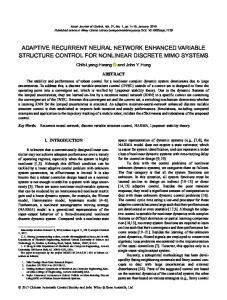
Fig. 1. The structure of the ESN and readout system. On the left, the input signal is fed into the reservoir network through the fixed weights Win . The reservoir network recodes these, and the output from the network is read out using the readout network on the right.

clear from the exponentially increasing number of publications in recent years. Another way to look into the ESN concept would be as follows. ESN is mapping the input vector to a higher dimension using randomly generated RNNs with forgetting memory and using the teaching signal in learning a simple linear classifier in the output layer. However, this means that a very big reservoir is needed to find the desired linear hyperplane that separates the different classes. This leads to the need to use an extremely large reservoir size (using reservoir of size 10000 is not uncommon in ESN) to achieve state-of-the-art performance [19]. In addition, applying a linear read-out function would mean that mapping to such a high dimension would emphasise the need for a bigger data sample size and more advanced regularisation techniques as in some cases the size of the reservoir will be much bigger than the number of training samples. The previous description is similar to SVMs; however, the nature of SVMs allows them to deal with infinite space without suffering from the same issues. The shared similarity between ESN and SVMs will be discussed in the next section along with an overview of the nature of SVMs. B. Support vector machines The support vector machine was developed by Vapnik in the late 1990s and since then its popularity has grown rapidly. This is mainly because it achieves state-of-the-art performance in many real-world applications and generalises well on unseen data. Another important factor is that, unlike neural networks, SVMs provide reproducible results. In addition, error bounds can be relatively easy to compute, and these offer guidance on the model generalisation performance. The main concept of SVMs is mapping the input vector to a higher dimension feature space and finding the optimal hyperplane that separates the two classes by maximising the margin [17]. Only a subset of the training data points are selected, known as support vectors, hence the name. Several support vectors are used in estimating the generalisation performance; the number decreases as the number of support vectors increases. Mapping from the input space to the feature space is accomplished by using the kernel trick, which provides a mapping to a high space dimensional without the need to specifically visit this space. The kernel can be defined as any function that satisfies Mercer’s theorem [7]. The radial basis kernel and linear kernel are among the most widely used kernels with SVMs. However, developing new kernels

that express the similarity for different applications is an active research area and many kernels have been designed in recent years to tackle specific applications. SVMs were originally designed as binary classifiers so different techniques are being used to extend SVMs to the multi-class problem. The main approaches are ’one against all’ (OAA) and ’one against one’(OAO) where in the first approach N SVM classifiers will be built, one for each class, and (N 21)N binary SVMs classifiers are implemented; the majority voting among these classifiers will be used in predicting new points citemulticlass support vector machines [14]. The main equation of SVMs that is used to estimate the decision function from a training dataset [7]:is as follows:

f (x) = sign

l X

yn ↵n .k(x, xn ) + b

n=1

!

(4)

where l is the number of the support vectors, b is the bias term, yn 2 { 1, +1} is the class sign to which the support vector belongs and ↵ is obtained as the solution of the following quadratic optimisation problem: p P min 12 wT w + C ⇠i i=1

s.t yi (w ⇠i

T

(xi ) + b)

1

⇠i

0, i = 1, ...p

The number of support vectors cannot be greater than the number of the data points in the dataset; ideally, it should be a relatively small fraction of the dataset. The major limitation of SVMs is the lack of ability to handle dynamic systems. This can be addressed by converting time series to fixed long vectors before applying SVMs. However, this approach can make the resulting vectors very long, resulting in the curse of dimensionality severely affecting performance. III.

P ROPOSED APPROACH (ESN & SVM S )

We present and motivate a detailed description of the proposed model. However, the strengths and weaknesses of this approach will be fully discussed in the Result & Discussion. The main motivation behind the development of this model is that the linear read-out function used in the output layer in ESN has very limited classification ability. This means that to achieve state-of-the-art performance, a huge reservoir needs to be used in many real-world applications to find a feature space where the different classes are linearly separable. This may be problematic as it can lead to dealing with a regime where the number of degrees of freedom is much bigger than the sample size and applying the simple linear read-out function to calculate the output weights may result in severe over-fitting. The generalisation error bounds will also not be valid in such regime. In addition, linear read-out is sensitive to outliers, which means that noisy data can severely affect the performance. Another issue that arises from applying the simple read-out function is that it is possible to end up with a non-invertible matrix as a response to the reservoir dynamic, which leads to several issues in learning the final weights in the output layer. Based on the previous argument, we suggest

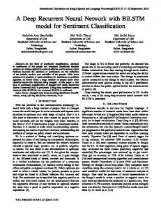
Fig. 2.

The proposed system Structure

replacing the simple linear read-out function with SVMs, as described below. First, mapping the input vector to higher dimensions using Win , which is a p by r matrix where p is the dimension of the input vector and r is the reservoir size, means that it can be initialises randomly, similar to ESN. Then constructing the reservoir randomly Wres , which is an r by r matrix, is applied in the same manner as in ESN and collects the response of the reservoir in Xcollected , which is a matrix m by r where m is the number of samples. This matrix Xcollected with the target label ~y is used to train SVMs, which is a vector of m components where ith element represents the class label for the ith sample in the training set. To predict a new data point, it is necessary to map using Win and Wres , and feed the output to the trained SVMs to determinate the class label of the sample. A summary of these steps is provided below: •

Step 1: Map the input signal using Win in and pass it to the reservoir the reservoir Wres for time 0.

•

Step 2: Repeat the same procedure until the end of the signal (different samples do not need to be the same length) and collect the response of the reservoir in Xcollected .

•

Step 3: Use Xcollected and target label ~y to train single SVM classifiers in the binary classification problem or multiple SVM classifiers in the multiclassification problem.

•

Step 4: Predict a new data point by using the mapping procedures described in steps 1 and 2 and applying the learned SVM classifiers on the response of the network to determine the label of the new sample.

To optimise the parameter of the reservoir and SVMs, we suggest using a validation set to optimise the hyperparameters of an ESN. Once this has been accomplished, the output of a reservoir with the same parameters estimated in the previous step is used to select SVM parameters such as the kernel type and the cost function based on their performance on the validation set. These steps usually help in reducing the time needed in optimising the proposed approach, especially when dealing with multiple label classification tasks. IV.

E XPERIMENT

To evaluate the performance of the suggested approach, a real-world application task was selected: Automated Arabic

Speech Recognition. Automated speech recognition (ASR) is concerned with the development of computational models that allow computers to map from acoustic signals to a string of words. Although this task can be performed extremely well by humans, developing a system to perform even a relatively simple ASR task such as recognising the digits from 0 -9, widely known as the Digits Task, is a challenge, especially with noisy data. Several techniques have been developed to tackle this problem; however, by far the most widely adopted has been the hidden Markov model (HMM). In recent years, this has started to change, however, as attention in the field has begun to shift towards the adaptation of the recurrent artificial neural network (RANN) [18]. A comparison was carried out among ESN, ESNSVMs and the state-of-the-art performance models developed by Hammami et al. (2011) [6] and P. R. Cavalin et al. (2012) [1].To obtain a comparable result, the same dataset used by Hammami and P. R. Cavalin, the well-known Arabic spoken digits, was used to develop and test the system. A. Dataset In this experiment, the Arabic spoken digits dataset was used; this dataset was developed at the laboratory of automatic and signals of the University of Badji-Mokhtar - Annaba, Algeria [4]. This ensures a fair comparison with the stateof-the-art methods as it was evaluated on this same dataset. The Arabic spoken digits dataset contains the Arabic digits 09, with each digit spoken 10 times by 88 native speakers, 44 males and 44 females. Thus, it contains 8800 samples which are divided as follows: 6600 instances for training and 2200 instances for testing. The training set was divided into two parts with one used for training, which contains almost 75% of the training sample (5000 samples), and the other used as a validation set (contains 1600 samples) in the model selection phase. Here, we report the result on the test data, which was not used in the development process of the model. The dataset was recorded at a sampling rate of 11025 Hz 16 bits, and 13 Melfrequency cepstral coefficients (MFCC) were extracted using a hamming window and filter pre-emphasized: 0.97. Matlab code was written to implement ESN and the LIBSVM library [2], the Matlab version, was applied to train SVM classifiers in the output layer of ESNSVMs. V.

R ESULT & D ISCUSSION

In this section, the result of the conducted experiment will be described. In addition, the selection of the systems parameters will also be fully stated and the chosen parameters used in the final model will be specified to ensure the reproducibility of the reported result. A comparison of performance between the developed model and two of the state-of-the-art approaches reported in the literature will also be included. The properties of the model will be discussed along with the regime in which the model is most likely to achieve its full potential. Finally, the limitation of this approach will also be discussed, which can provide useful guidance on how to improve the suggested model. Parameter selection lies under the umbrella of the model selection phase and techniques vary in their sensitivity to changes of the hyperparameters. RNNs are known to be

English

Arabic Sounds

Zero

Arabic

TM

ESNSVMs

.sifr

93.28

98.6

One

wahid

99.95

97.7

Two

itnan

90.19

97.7

Three

talatah

92.16

98.6

Four

arbaa

94.59

96.3

Five

hamsah

97.62

98.6

Six

sittah

95.35

95

Seven

saba

89.27

93.6

Eight

tamaniyyah

92.98

99

Nine

tisah

95.51

99

94.04

97.45

Average

TABLE I.

Fig. 3.

T HE RESULT OBTAINED BY ESNSVM S FOR EACH DIGITS COMPARED WITH TM APPROACH

A comparison among ESNSVMs, LoGID and TM

sensitive to weight initialisation, which limits the ability to reproduce the result even when using similar architecture. On the other hand, SVMs are more robust to changes in the initial weights and reproducibility is more likely when fixing the kernel type and the regularisation parameter, mainly due to convex optimisation which results in a global minimum solution. The hyperparameters of each model tend to affect the overall performance differently, which leads researchers to focus on the most important according to their impact. The typical method of selecting hyperparameters, which is also adopted in this experiment, is to use a subset of the training set, which is known as a validation set, in testing a variety of hyperparameter values. The values corresponding to the best result on

the validation set will be selected. Once the hyperparameters are fixed, the model is tested on the test dataset and results are reported and compared with other approaches. ESN has several hyperparameters that need to be set empirically using the validation set; however, their impact on the performance varies significantly. The two major hyperparameters that need to be determined are the reservoir size and the leakage rate as they both have a major impact on the performance. Finding the optimal value that maximises the performance may require a sound background in machine learning as using a very large reservoir may easily result in high variance, which needs to be addressed by adopting the appropriate regularisation technique. In determining the leakage rate, prior knowledge of the nature of the task dynamic is useful. In this experiment, using a leakage rate value larger than 0.4 prevents the model from distinguishing among the Arabic digits 4,7 and 9 as they all end with the same sound. The other hyperparameter is the scaling constant, which is optimised to obtain the desired dynamic of reservoir. However, the literature has reported that it does not affect the performance severely; the same was observed in this experiment. ESNSVMs seems to be less sensitive to changes in the leakage rate than ESN; however, the leakage rate is still a dominant hyperparameter in both models. In ESNSVMs, there is also a need to set the hyperparameters of the SVM models, which include the kernel selection, the regularisation parameter and the epsilon value. The values used in ESN are: reservoir size is 900, leakage rate is 0.005 and scaling constant is 1.75. In ESNSVMs, the same previous parameters and the RBF kernel are applied with gamma 0.001 and the cost value is 1000, known as the regularisation parameter. Systems

Accuracy Rate

TM (Nacereddine Hammami et al, 2011) [6]

94.04%

LoGID ( Paulo R. Cavalin et al,2012) [1]

95.99%

TABLE II.

Echo State Network

96.91%

Proposed System (ESNSVMs)

97.45 %

T HE RESULTS OBTAINED BY THE PROPOSED SYSTEM , ESN AND FROM THE TWO COMPARED STUDIES

The performance of both ESN and ESNSVMs is superior to the published results of the state-of-the-art techniques found in the literature. Our result is presented in table 2, which clearly shows the robustness of these two approaches compared to the other models. The comparison is also valid as all the compared studies used the same dataset in developing their model and reported the performance on the provided test dataset. This means the performance of all the models, including this model, was reported based on the same 2200 samples, representing 25% of the dataset size, which were divided by the developer of the dataset. In addition, the test data have not been used in training the model or in selecting its hyperparameters. ESNSVMs maintains a higher accuracy rate than ESN and the gap between their performance peaks when using a very small reservoir size. The maximum difference reported is 15% when the size of the reservoir is equal to the size of the input signal dimension. Based on the previous obtained result, we argue that using ESNSVMs can improve system performance. Moreover, it is clear from our experiment that when using a small to medium

Fig. 4. The effect of the Reservoir Size on the Performance of ESN and ESNSVMs.

Fig. 5.

Confusion matrix of best result obtained by ESNSVMs

reservoir size ESNSVMs achieves a significant improvement in the accuracy rate. This particularly could be attractive when dealing with time series with a very high dimension i.e. image sequences. Also, the ESNSVMs shows robust performance against over-fitting with easily computed error bounds of the SVMs, which offers an estimation of the model’s generalisation ability. Developing new kernels to tackle a specific problem is also enabled when using ESNSVMs, which may lead to improvements in performance on different tasks. The suggested model has some limitations that could prevent it from achieving the desired performance in certain regimes. The main limitation of ESNSVMs is the added complexity over ESN, which is represented in the need to optimise. The suggested model has some limitations that could prevent it from achieving the desired performance in certain regimes. The main limitation of ESNSVMs is the added complexity over ESN, which is represented in the need to optimise SVMs parameters used in the output layer. This include the choice of kernel and its associated parameters. The learning in general will take longer time specially when applying ESNSVMs on multiple class problems with medium to large numbers of classes. This due to the nature of SVMs which is a binary classifier requires constructing at least equal to the number of problem classes , in the one against all approach. This limits the ability of ESNSMs in dealing with multi-class classification problem with medium to large number of classes. VI.

C ONCLUSION

We have proposed the ESNSVMs approach, which combines ESN and SVMs for time series classification. To evaluate the performance of the ESNSVMs, we conducted an experiment on the well-known Arabic spoken digits. The dataset is publicly available and contains 8800 samples for Arabic digits 0-9. The result has been compared with ESN and two other

state-of-the-art models. ESNSVMs achieves a high accuracy rate of 97.45%, which demonstrates the potential of applying ESNSVMs on multi-class time series classification problems with a small number of classes. In addition, the proposed approach achieves a higher accuracy rate than ESN, especially when the size of the reservoir size is small. Further work will include validating ESNSVMs on different classification tasks, i.e. handwritten classification and different datasets. The model complexity of the output layer should be reduced to give ESNSVMs the ability to handle multi-class classification problems with large numbers of classes. In addition, model performance should be tested on noisy data; this task is known to be challenging for traditional approaches, such as HMM, which generally obtains a poor result. ACKNOWLEDGMENT We wish to acknowledge Al Imam Mohammad Ibn Saud Islamic University (IMSIU) for the financial support for this work. . R EFERENCES [1]

[2] [3] [4] [5] [6] [7] [8] [9] [10] [11] [12] [13] [14]

[15]

P. R. Cavalin, R. Sabourin and C. Y. Suen, ”LoGID: An adaptive framework combining local and global incremental learning for dynamic selection of ensembles of HMMs,” Pattern Recognit, vol. 45, pp. 35443556, 9, 2012. C. C. Chang and C. J. Lin, ”LIBSVM: a library for support vector machines,” ACM Transactions on Intelligent Systems and Technology (TIST), vol. 2, pp. 27, 2011. Chih-Wei Hsu and Chih-Jen Lin, ”A comparison of methods for multiclass support vector machines,” Neural Networks, IEEE Transactions on, vol. 13, pp. 415-425, 2002. A. Frank and A. Asuncion, ”UCI Machine Learning Repository,” 2010. A. Graves and J. Schmidhuber, ”Offline handwriting recognition with multidimensional recurrent neural networks,” in 2008, pp. 545-552. N. Hammami and M. Bedda, ”Improved tree model for arabic speech recognition,” in Computer Science and Information Technology (ICCSIT), 2010 3rd IEEE International Conference on, 2010, pp. 521-526. M. A. Hearst, S. T. Dumais, E. Osman, J. Platt and B. Scholkopf, ”Support vector machines,” Intelligent Systems and their Applications, IEEE, vol. 13, pp. 18-28, 1998. S. Hochreiter and J. Schmidhuber, ”Long short-term memory,” Neural Comput., vol. 9, pp. 1735-1780, 1997. H. Jaeger, ”The echo state approach to analysing and training recurrent neural networks-with an erratum note,” Tecnical Report GMD Report, vol. 148, 2001. M. Lukosevicius, ”A Practical Guide to Applying Echo State Networks,” Neural Networks: Tricks of the Trade, pp. 659-686, 2012. W. Maass, T. Natschl?ger and H. Markram, ”Real-time computing without stable states: A new framework for neural computation based on perturbations,” Neural Comput., vol. 14, pp. 2531W. S. McCulloch and W. Pitts, ”Neurocomputing: Foundations of research,” in , J. A. Anderson and E. Rosenfeld, Eds. Cambridge, MA, USA: MIT Press, 1988, pp. 15-27. W. McCulloch and W. Pitts, ”A logical calculus of the ideas immanent in nervous activity,” Bull. Math. Biophys., vol. 5, pp. 115-133, 12/01, 1943. J. Milgram, M. Cheriet and R. Sabourin. One against one or One against all: Which one is better for handwriting recognition with SVMs? Presented at Tenth International Workshop on Frontiers in Handwriting Recognition. 2006, . J. B. Pollack, ”Connectionism: Past, present, and future,” Artif. Intell. Rev., vol. 3, pp. 3-20, 1989

[16]

J. J. Steil, ”Backpropagation-decorrelation: Online recurrent learning with O (N) complexity,” in Neural Networks, 2004. Proceedings. 2004 IEEE International Joint Conference on, 2 [17] V. N. Vapnik, ”An overview of statistical learning theory,” Neural Networks, IEEE Transactions on, vol. 10, pp. 988-999, 1999. [18] D. Verstraeten, B. Schrauwen and D. Stroobandt, ”Reservoir-based techniques for speech recognition,” in Neural Networks, 2006. IJCNN ’06. International Joint Conference on, 2006, pp. 1050-1053. [19] D. Verstraeten, ”Reservoir Computing: computation with dynamical systems,” pp. , 178, 2009.