A Novel Approach to Design Classifiers Using Genetic Programming

IEEE TRANSACTIONS ON EVOLUTIONARY COMPUTATION, VOL. 8, NO. 2, APRIL 2004

183

A Novel Approach to Design Classifiers Using Genetic Programming Durga Prasad Muni, Nikhil R. Pal, Senior Member, IEEE, and Jyotirmoy Das

Abstract—We propose a new approach for designing classifiers 2) problem using genetic programming (GP). for a -class ( The proposed approach takes an integrated view of all classes when the GP evolves. A multitree representation of chromosomes is used. In this context, we propose a modified crossover operation and a new mutation operation that reduces the destructive nature of conventional genetic operations. We use a new concept of unfitness of a tree to select trees for genetic operations. This gives more opportunity to unfit trees to become fit. A new concept of OR-ing chromosomes in the terminal population is introduced, which enables us to get a classifier with better performance. Finally, a weight-based scheme and some heuristic rules characterizing typical ambiguous situations are used for conflict resolution. The classifier is capable of saying “don’t know” when faced with unfamiliar examples. The effectiveness of our scheme is demonstrated on several real data sets. Index Terms—Classifier, genetic programming (GP), multicategory pattern classification, multitree representation, nondestructive directed point mutation, OR-ing operation.

I. INTRODUCTION

G

ENETIC PROGRAMMING (GP) introduced by Koza and his group [1] is popular for its ability to learn relationships hidden in data and express them automatically in a mathematical manner. GP has already spawned numerous interesting applications such as [2]–[12]. GP has been used by many authors [13]–[18] to design classifiers or to generate rules for two class problems. Although genetic algorithm has been used by many researchers to design classifiers for multiclass problems, only a few attempts have been made to solve the same problem using GP. Holland [19] provides a nice discussion about designing classifier systems. Rauss et al. [13] used GP to evolve binary trees (equations) involving simple arithmetic operators and feature variables for hyper-spectral image classification. A data point is assigned a class if the response for that class is positive and responses for all other classes are negative. Agnelli et al. [14] also applied GP for image classification problems. In addition to simple arithmetic operations, they considered exponential function, conditional function and constants to construct binary trees. The generation of rules using GP for two class problems has been addressed by Stanhope and Daida [15] and Falco et al. [16]. Binary trees consisting of logical functions, comparators, feature variables and constants have been generated to represent possible classification rules. During the construction of binary trees, some

Manuscript received August 30, 2002; revised June 9, 2003. The authors are with the Electronics and Communication Sciences Unit, Indian Statistical Institute, Calcutta 700108, India (e-mail: [email protected]; [email protected]; [email protected]). Digital Object Identifier 10.1109/TEVC.2004.825567

restrictions are imposed to enforce a particular structure, so that they can represent logical statements or rules. Dounias et al. [17] implemented GP to generate both crisp and fuzzy rules for classification of medical data. Multicategory pattern classification using GP has been attempted by a few researchers [12], [20]–[22]. Loveard et al. [20] proposed five methodologies for multicategory classification problems. Of these five methodologies, they have shown that dynamic range selection method is more suitable for multiclass problems. In this dynamic range selection scheme, they record the real valued output returned by a classifier (tree or program) for a subset of training samples. The range of the recorded to repvalues is then segmented into regions resent class boundaries. If the output of the classifier for a pattern falls in the region , then the th class is assigned to . Once the segmentation of the output range has been performed, the remaining training samples can then be used to determine the fitness of an individual (or classifier). Chien et al. [21] used GP to generate discriminant functions using arithmetic operations with fuzzy attributes for a classification problem. In [22], Mendes et al. used GP to evolve a population of fuzzy rule sets and a simple evolutionary algorithm to evolve the membership function definitions. These two populations are allowed to co-evolve so that both rule sets and membership functions can adapt to each other. For a -class problem, the system is run times. Kishore et al. [12] proposed an interesting method which considers a class problem as a set of two-class problems. When a GP classifier expression (GPCE) is designed for a particular class, that class is viewed as the desired class and the remaining classes taken together are treated as a single undesired class. So, with GP runs, all GPCEs are evolved and can be used together to get the final classifier for the -class problem. They have experimented with different function sets and incremental learning. For conflict resolution (where a pattern is classified by more than one GPCE) each GPCE is assigned a “strength of association” (SA). In case of a conflicting situation, a pattern is assigned the class of the GPCE having the largest SA. They have also used heuristic rules to further reduce the misclassification. Lim et al. presented an excellent comparison of 33 classification algorithms in [23]. They used a large number of benchmark data sets for comparison. None of these 33 algorithms use GP. The set of algorithms includes 22 decision tree/rule-based algorithms, nine statistical algorithms, and two neural networkbased algorithms. We shall use the results reported in [23] for comparison of our results. In this paper, we propose a method to design classifiers for a -class pattern classification problem using a single run of GP. For a class problem, a multitree classifier consisting of trees

1089-778X/04$20.00 © 2004 IEEE

184


is evolved, where each tree represents a classifier for a particular class. The performance of a multitree classifier depends on the performance of its constituent trees. A new concept of unfitness of a tree is exploited in order to improve genetic evolution. Weak trees having poor performance are given more chance to participate in the genetic operations so that they get more chance to improve themselves. In this context, a new mutation operation called nondestructive directed point mutation is proposed which reduces the destructive nature of mutation operation. During crossover, not only is swapping of subtrees among partners performed but also swapping of trees is allowed. As a result, more fit trees may replace the corresponding less fit trees in the classifier. Multiple classifiers from the terminal population are then combined together by a suitable OR-ing operation in order to further improve the classification result. A conflict situation occurs when a pattern is recognized by more than one tree to their respective classes. Each tree of the classifier is assigned a weight to help conflict resolution. In addition, heuristic rules, that characterize typical situations when the classifier fails to make unambiguous decisions, are used to further enhance the classifier performance. For a reasonably large number of training points, if the classifier fails to make unambiguous decision, and the response of the classifier for each such data point is the same, then it is likely that those training points come from some particular area of the input space. Heuristic rules exploit this information and try to resolve situations when more than one tree of the classifier produce positive responses. A combination of all of these results in a good classifier.

Step 3) A genetic operator is selected probabilistically. Case i) If it is the reproduction operator, then an individual is selected (we use fitness proportionbased selection) from the current population and it is copied into the new population. Reproduction replicates the principle of natural selection and survival of the fittest. Case ii) If it is the crossover operator, then two individuals are selected. We use tournament selection where number of individuals are taken randomly from the current population, and out of these , the best two individuals (in terms of fitness value) are chosen for the crossover operation. Then, we randomly select a subtree from each of the selected individuals and interchange these two subtrees. These two offspring are included in the new population. Crossover plays a vital role in the evolutionary process. Case iii) If the selected operator is mutation, then a solution is (randomly) selected. Now, a subtree of the selected individual is randomly selected and replaced by a new randomly generated subtree. This mutated solution is allowed to survive in the new population. Mutation maintains diversity. Step 4) Continue Step 3), until the new population gets solutions. This completes one generation. Step 5) Unlike GA [25], GP will not converge. So, Step 2)–4) are repeated till a desired solution (may be 100% correct solution) is achieved. Otherwise, terminate the GP operation after a predefined number of generations.

II. BRIEF INTRODUCTION TO GP GP [1], [2], [24] evolves a population of computer programs, which are possible solutions to a given optimization problem, using the Darwinian principle of survival of the fittest. It uses biologically inspired operations like reproduction, crossover and mutation. Each program or individual in the population is generally represented as a tree composed of functions and data/terminals appropriate to the problem domain. The set of functions and set of terminals/inputs must satisfy the closure and sufficiency properties. The closure property demands that the function set is well defined and closed for any combination of arguments that it may encounter. On the other hand, the sufficiency property requires that the set of functions in and the set of terminals be able to express a solution of the problem [1]. The function set may contain standard arithmetic operators, mathematical functions, logical operators, and domain-specific functions. The terminal set usually consists of feature variables and constants. Each individual in the population is assigned a fitness value, which quantifies how well it performs in the problem environment. The fitness value is computed by a problem-dependent fitness function. A typical implementation of GP involves the following steps. Step 1) GP begins with a randomly generated population of solutions of size . Step 2) A fitness value is assigned to each solution of the population.

III. PROPOSED MULTITREE GP-BASED CLASSIFIER , where is A classifier D is a mapping, is the set of label vectors the -dimensional real space and for a -class problem and is defined as . For any vector , is a vector in -dimension with only one component as 1 and all others as 0. In other words, a classifier is a function which takes a feature vector in dimension as input and assigns a class label to it. In this paper, our objective is to find a using GP. We shall use a multitree concept for designing classifiers. The beauty of using this concept is that we can get a classifier for the multiclass problem in a single run of GP. Given a set of training data and its associated set of label vectors , our objective is to find a “good” using GP. For a two class problem, a possible classifier or an individual is generally represented by a single tree ( ). For a pattern if else

class class

The single tree representation of the classifier is sufficient for a two-class problem. This scheme can be extended to a multicategory classification problem. In our design, every chromosome

MUNI et al.: NOVEL APPROACH TO DESIGN CLASSIFIERS USING GENETIC PROGRAMMING

or individual will have a tree for every class. So, the th chro, mosome will have trees, and these will be denoted by . If the identity of the chromosome is not important, then for clarity we will ignore the superscript and use only the class index, i.e., the subscript. So a possible solution or an . individual for the GP is represented by trees For a pattern if

and then

for all .

, ,

If more than one tree show positive responses for the pattern , then we require additional methodologies for assigning a class to . The steps followed to achieve our goal are summarized in the following sections. A. Initialization Each of the trees for each individual is initialized randomly using the function set which consists of arithmetic functions containing feature variables and conand the terminal set stants. The function set and terminal set used here are as follows: and feature variables , where R contains randomly generated constants in [0.0,10.0]. We have initialized trees using the ramped half-and-half method [1]. B. Training and Fitness Measure The GP is trained with a set of training samples, . Instead of training the GP with all training samples at a time, it is accomplished in a step-wise manner increasing the number of training samples in steps. The step-wise increment of training samples is accomplished by a . The step-wise learning can preset number of generations reduce the computational overhead significantly [27], [28] and steps, then can improve the performance [12]. If we use generations. And the incremental each step size will be change in the size of training subset in each step will be . Let be the set of the training samples at step , . At the first step and at the last step, . After step-wise learning GP is continued with all N training samples up to the maximum number of generation . M, where While training, the response of a tree for a pattern is expected to be as follows: if if

class class

In other words, a classifier with trees is said to correctly classify a sample , if and only if all of its trees correctly classify that sample. We emphasize that if a training sample is correctly classifies , if from class , then we say that tree

185

. On the other hand, the tree is said to correctly . For each correct classification of a classify , if training sample by a classifier, its raw fitness is increased by 1. At the initial stage of learning (evolution), if some but not all of the trees of a classifier are able to do a good job, then that should not necessarily be considered a bad classifier. Because by giving more chance to unfit trees to take part in subsequent genetic operations, unfit trees may be made to converge to more fit trees and, hence, may result in a better overall classifier. We will take into account this factor, while computing the fitness value. Let trees correctly classify a training sample . Then, we increase the raw fitness by irrespective of the class label of . In other words, we give equal importance to all trees. So, if all trees correctly classify a data point, then the raw fitness is increased by 1 as mentioned above. This partial increment (for ) is considered only of raw fitness function by generations. during the stepwise learning, i.e., only up to This helps to refine the initial population. After completion of the step-wise learning, the fitness function considers only the correctly classified samples. We again emphasize the definition is from class , of correct classification by a tree. If , then ’s classification then for a chromosome, if , then also classifies is correct, and also, if correctly. . Let be the number of trees that correctly classify So the fitness function at step of the step-wise learning task is defined as (1) Number of training samples used at In (1), step . After step-wise learning we consider the samples which are of the classifier. So, the correctly classified by all trees fitness function after step-wise learning is defined as shown in (2), at the bottom of the page. Thus, during initial evolution, individuals with potential (partially good) trees are given some extra importance in the fitness calculation. Note that fitness function (1) or (2) can be used for selection of individuals. Algorithm fitness shows the procedure for evaluating the fitness of an individual during the step-wise learning process. Algorithm fitness BEGIN ; for all for all ; if ( end if

/

AND ) ; if classifies

Number of training samples correctly classified for which

(2)

186


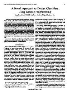
Fig. 1. (a) and (b) Chromosomes C1 and C2 before crossover operation. (c) and (d) Chromosomes C1 and C2 after crossover operation.

correctly if (

D. Modified Crossover Operation

/

AND ) ; classifies end if / if correctly / / For other cases the trees make is not wrong decisions and, hence, incremented / end for ; end for ; END C. Unfitness of Trees When all trees are able to classify a pattern correctly then the said classifier will recognize the pattern correctly. On the other hand, if there are some unfit trees in the classifier, they should be given more chance to evolve through genetic operations in order to improve their performance. In addition to the fitness functions, we need another unfitness function, to select a tree after an individual is selected [using (1) or (2)] for genetic operations. So after an individual is selected for genetic operation, we compute the degree of unfitness of its each constituent tree , . The total number of training samples for which is unable to classify correctly is counted. Let be the total number of training samples not correctly classified by . To compute , , we proceed as follows: If a training , then is increased by sample is from class and , then is increased by 1. 1 and also if If , then is more unfit then . Let

(3) This is used as the probability of selection of the th tree by the Roulette wheel selection as an unfit tree for genetic operations as described in Sections III-D and E. In this way, the unfit trees are given more chance to take part in the genetic operations to rectify themselves.

Crossover plays a vital role in GP for evolution. To select trees (within a chromosome) for crossover, we use as the probability of selection and this gives more preference to unfit trees for the crossover operation. We use the tournament selection scheme for selecting chromosomes for the crossover operation. The fitness function defined in (1) or (2) is used for the selection of a pair of chromosomes. Let the selected chromosomes be and . Each of and has trees , , . from chromosome using Now, we select a tree , Roulette wheel selection based on the probability . is computed using (3). We now randomly and , where the probability select a node from each of and that of a terminal of selecting a function node type is . After selecting one node from node type is , each of the two trees and , we swap the subtrees rooted at the selected nodes. In addition to this, we also swap the trees and for all . That means we swap trees of chromosome with of chromosome for all . This crossover operation has three interesting aspects. First, we swap subtrees between classifiers from the same class. The motivation is that, good features of one classifier may get combined with good features of another classifier. Note that a subtree of the good classifier for class , may not be very useful of a different classifier. The second interfor a class , esting aspect of this crossover operation is that it also exchanges classifier trees as a whole between two chromosomes. The third point is that, by selecting trees for the crossover operation according to their unfitness, the chance of unwanted disruption of already fit trees is reduced and the chance of evolution of weak trees is increased. Thus, we not only try to change weak trees but also try to protect good trees from the destructive nature of the crossover operation. Fig. 1 illustrates the crossover operation. In Fig. 1(a) and (b), of two chromosomes are selected for crossover. Suppose is selected using (3). A node of and a node of (shown by the dotted circles) are then randomly selected (the probability of selecting a function node is , and that of a terminal node is ) for crossover operation. Now, the subtrees rooted at the are swapped, selected nodes are swapped. Also, . The resultant chromosomes obrespectively, with tained after crossover are shown in Fig. 1 (c) and (d).


A schematic description of the crossover operation is given next. Algorithm Crossover Step 1) Randomly select (tournament size) individuals from the population for tournament selection. Step 2) Select the best two individuals and , say) of the tournament ( for the crossover operation. , of using Step 3) Compute (3). of , by the Step 4) Select a tree Roulette-wheel selection using the . unfitness probability, Step 5) Choose a node type—a function (internal) node type is chosen and a terminal with probability (leaf) node type is selected with probability . Randomly select a node of the chosen type from each and . of the trees Step 6) Swap the subtrees rooted at the and . selected nodes of with , for all Step 7) Swap . E. Modified Point Mutation Operation The conventional GP mutation is usually a destructive process, because it swaps a subtree for a randomly generated tree. For this reason, we have utilized point mutation with some additional precautions. It is just like the fine-tuning of a solution. In case of point mutation, a node is randomly picked. If it is a function (terminal) node then it is replaced by a randomly chosen new function (terminal) node (having the same arity). Thus, it causes a very small change. To make a considerable change, it is repeated a number of times. Although, usually it is not expected to severely affect the tree, sometimes its effect could be significant. So, we introduce a kind of directed mutation, which always accepts mutations that improve the solution, but also occasionally, with some probability, accepts a mutation that does not improve the solution. This involves comparison of the fitness of the mutated tree with that of the original tree. To of the mutated reduce computation time, we evaluate fitness and fitness of original tree using only 50% of tree equals , then we the training samples of the th class. If use the remaining 50% of training samples of the th class to find . If the mutated tree is equal or more fit than the original tree, then the mutated tree is retained. Otherwise, it is ignored . with probability th. We have taken th Mutation causes random variation and unfit trees need such variation more than fit ones. Consequently, after selecting an individual for mutation, the more unfit trees are given more chances to mutate. In other words, more fit trees are given more opportunities to protect themselves from the destructive nature of mutation. To achieve this, we proceed as follows. We randomly select a chromosome and then select a tree from the chromosome. The tree is selected using Roulette wheel

187

in (3). This is tree selection with a selection criterion with probability proportional to the unfitness of the tree. Then, we select % of nodes from the selected tree for point mutation. and a terminal A function node is selected with probability , . node is selected with probability After mutation, a decision is made as to whether the mutated tree will be retained or ignored. This procedure is repeated times for the selected individual. The basic steps of the point mutation are schematized in Algorithm Mutation. Algorithm Mutation Step 1) Randomly pick an individual(C) for mutation (from the old population). Step 2) Compute unfitness probability , of C using (3). Step 3) Select a tree of with Roulette wheel selection using , . Step 4) Randomly select a node from with probability of selecting a and that of a function node for point mutaterminal node tion. Step 5) If the selected node is a function node, replace it with a randomly chosen function node (having the same arity). Otherwise, replace it with a randomly chosen terminal node. Step 6) Repeat Step 4) and Step 5) for % . of the total nodes in Step 7) Evaluate the fitness of the of mutated tree and fitness the original tree using 50% of training samples of the th class. Step 8) If then evaluate again and using the remaining 50% of training samples of the th class. then accept the mutated Step 9) If tree, else retain it with probability 0.5. Step 10) Repeat Step 3) through Step 9) times. F. Termination of GP The GP is terminated when all training samples are classified correctly by a classifier (an individual of the GP populaof generations are completed. tion) or a predefined number training samples are correctly classified by the If all of the GP, the best individual (BCF) of the population is the required optimum classifier CF. Otherwise, when the GP is terminated after completion of M generations, the best individual (BCF) of the population is passed through an OR-ing operation to obtain the optimal classifier CF. The best individual (BCF) is selected as follows. number of correctly classified training samples Let hit by the classifier . The individual which scores the maximum

188


is considered the best classifier BCF. If more than one individual score the same hit (maximum), then the individual which has the smallest number of nodes is chosen as the best individual BCF.

chromosomes then we In this way, if the population has , combined classifiers. will get The combined classifier which correctly classifies the maximum number of training samples, is taken as the resultant classifier CF.

G. Improving Performance of Classifier with OR-ing It is possible that the terminal GP population contains two and chromosomes such that is good for a parmodels well anticular segment of the feature space, while other segment of the feature space. The overall performance, in and could be comparable terms of misclassification, of or different. In this case, combining and by OR-ing may result in a much better classification tree. This is the principle behind this OR-ing operation. The best individual BCF of the GP run, which is unable to classify correctly all training samples is further strengthened by this operation. BCF is OR-ed in a consistent fashion with every individual of the terminal population. From this set of (OR-ed) pairs, the best performing (in terms of number of misclassifications) pair is taken as the optimum classifier CF. However, OR-ing is to be done carefully. Next, we explain how the OR-ing is done. We introduce a set of for the best chromosome indicator variables , BCF as if otherwise where In other words, if the th tree of BCF shows a positive response for a sample , then for that sample is 1; otherwise, it is 0. Now, to combine the BCF with any other chromosome , as we define another set of indicators , if otherwise For notational clarity, we consider a set of indicators using BCF and represent the combined classifier

to

.. .

The combined classifier is, thus, defined by . Given a data point , assigns a class label to as follows. If

and then

, for all .

and i,

H. Conflict Resolution The resultant classifier CF, thus obtained, is now ready for validation with the test data set. For a test data point , to make and an unambiguous decision, we need (or and ), for some , . However, it can happen that more than one tree of CF show positive responses. In this case, we face a conflicting situation. To resolve it, we use a set of heuristic rules followed by a weighting scheme. The heuristic rule-based scheme described next is a slightly modified version of the rule proposed by Kishore et al. [12]. Extraction of the Rules: The classifier CF is used to classify all training samples. The objective of the heuristic rules is to identify the typical situations when the classifier cannot make unambiguous decisions and exploit that information to make decisions. Let be the number of unclassified training samples of class for which either two or more trees or none of the trees of CF show positive response. For each such unclassified sample , , we compute a response vector in dimension as follows: if otherwise As an illustration, consider a four-class problem, where a from class 1 is not classified by CF, betraining sample cause more than one tree show positive responses. Suppose , , and show positive responses, and shows a negative response for the training example. Then, the corresponding rewill be . Similarly, if a training sponse vector of class 1 is unclassified because all trees show negsample , then the ative responses, i.e., is . response vector classes, then there can be at most If there are possible distinct response vectors when the classifier fails to make a decision. Let these vectors be . Clearly, . The classifier may produce a particular vector for several data points from represents a typical conflicting class . If this is so, then or ambiguous situation for class when the classifier cannot make a decision. Since several training data points generated the same response vector, , it is likely that those training points came from some particular area of the input space and the classifier failed to model that area correctly. These points are expected (but not necessarily) to form a cluster in the input space. Therefore, for a test data point , if CF fails to classify unambiguously and the response vector corresponding to matches , then it may be reasonable to classify to the th a rule for conflict resolution. We emphasis class. We call that unless is supported by a sufficient number of instances,


we should not use as a rule for conflict resolution for class . In other words, the number of cases from class for which is produced should be large. Suppose, the response vector unclassified samples, is obtained for times. We of the to decide on the acceptance of may use a threshold on as a rule. Using such a threshold, may also become a rule for a different class, but a particular should be used as a rule for only one class. , we find the class for which So, for a is the maximum. Then, is used to represent a rule only for class . The difference of our rules from those of Kishore et al. [12] is that authors in [12] used a threshold on the percentage of training samples to pick up the rules, while we threshold on the number of samples. The reason for such a choice, as explained earlier, is that if any is supported by a reasonable number of points , it should be considered a rule, and thus is indepen. dent of the size of The heuristic rules are derived from the behavior of the classifier when it fails. So unless there are sufficient number of failure cases, the rules may not be useful. Based on a few ex.A periments with the training data we decided to use better strategy would be to use a validation set to decide on the value of . If the classifier fails to classify a pattern unambiguously and that pattern produces a response vector which matches a heuristic rule, then the class corresponding to that rule is assigned to that pattern. If there is no heuristic rule for that response vector, then the weight-based scheme discussed next is used to assign a class to the pattern. If there is no heuristic rule at all, then we directly use the weight-based scheme. Weighting Scheme: The classifier CF is used to classify all of ditraining samples. Now, we compute a matrix , where is the total number of cases such that mension the instance is from class , but the th tree of classifier CF shows a positive response, i.e., , . In other words, gives the number of data points from class for which the gives a positive response. Consequently, diagonal eletree ments of represent the number of cases correctly classified and the off-diagonal elements represent the number of misclassified cases by the trees. For an ideal classifier, the sum of all diagonal elements will be and the sum of all off-diagonal elements will be zero. gives the number of data points from Now, all classes except class for which . So, gives the number of data points from other classes which are wrongly represents the false positive classified to class by tree . cases. cases. The classifier CF will make mistake for these , then the tree can be held most (or at least, If significantly) responsible for the misclassification reported by the classifier CF. For a row in , the difference between the total number of patterns of class and the diagonal element indicates the number of cases from class for which tree did not predict the result correctly. In other words, is related to how tree failed to represent its own class. represents the false negative ; then the th tree is also a determinant cases. Let of the poor performance of classifier CF.

189

that provides Therefore, for a tree , we define a weight the relative importance of the tree in making a correct prediction as follows. For the th tree of the CF, we compute

where

Total number of training samples (4) . These weights can be used for resolution of conflict, when needed. For a test data point , if we find that CF identifies a conflict and give between classes and (in other words, both ; positive responses), then is assigned to class , if otherwise, is assigned to class . Note that, this weight scheme is different from the one used by Kishore et al. [12]. We recommend using the heuristic rules first because each heuristic rule represents a typical mistake, a scenario represented by an adequate number of data points. Moreover, as pointed out by Kishore et al. [12], the weight-based scheme has some limitations. It cannot assign a class label, if none of the , . Also, in some cases, it may happen , and for another tree , that for with . Then, will be misclassified to class by the weight scheme. So, we suggest to use the heuristic rules first. If the heuristic rule cannot resolve the conflict, the weight scheme should be used. It is possible that neither the weight-based scheme nor the heuristic rule is able to assign a class label to a test data point. This must not be viewed as a disadvantage, but rather a distinct advantage. The classifier is able to say “don’t know” when faced with very unfamiliar examples. This is better than giving a wrong class. Moreover, if there are too many such “don’t know” cases, then these indicate that either the training set used was not a sufficient representative of the population that generated the data, or the identified classifier is a poor one. So, a redesign of the classifier is required. Note that the OR-ing operation, the heuristic rule generation, and computation of the weights are done only once after the GP terminates. Consequently, the additional computation involved for the postprocessing, as we shall see later, is much less than the time required for the GP to evolve. The complete algorithm is now schematized in Algorithm Classifier.

Algorithm Classifier BEGIN , , Let / of that generation and / till that / generation / Initialize population of size P for GP AND ) while ( if

190


Evaluate fitness of each individual using (1) else Evaluate fitness of each individual using (2). end if Find the best individual , . and if . end if Perform Breeding / perform all genetic operations / . / go to the next generation / end while / if all if training samples are classified correctly / else do OR-ing operation. end if Extract Heuristic rules and Compute using (4). weights END

Algorithm Breeding [32] BEGIN / of the Let next population / / / while Select one of the operators from reproduction, crossover and mutation , and , with a probability respectively. If (operator = reproduction) select an individual using fitness-proportion selection method and perform the reproduction operation. Now, . end if If (operator = crossover) select two individuals using tournament selection method and perform crossover. Now, . end if becomes , / Note that, if then reject the second offspring after crossover operation. / If (operator = mutation) select an individual randomly and . perform mutation. Now, end if end while END

I. Validation of Classifier After obtaining the classifier CF, it is necessary to validate it against test data sets. Each test data point is classified by the classifier CF. For a pattern , there are three possible cases. and for all other trees Case 1) For only one tree , or in case of the combined classiand all fier after OR-ing operation, only one other , . In this case, class is assigned to the pattern . This is the simplest case that does not require further operations. or more than one Case 2) For more than one tree are 1. Each tree for which or is called a competitive tree. To resolve this conflict or to assign only one class to the pattern , we first try to use the heuristic rules. If it cannot assign a class then we apply the weight-based scheme. Also, if there is no heuristic rule available, then we directly use the weight-based scheme. As an illustration, in , , a four-class problem, let and . In this case, and are the competitive trees and, hence, the vector will be . If there exists a heuristic rule which assigns class , , then that class is assigned to the pattern . Otherwise, the weight-based method will be tried. If , then class 3 will be assigned to , else class 4 will be assigned. Note that weights and rules will be computed only when the classifier CF makes mistakes on the training data set. So if CF makes 100% correct classification of the training data then weights and rules will not be available. or all . In this case, Case 3) For all trees none of the trees can recognize the pattern . So only the heuristic rules may resolve this situation. Here, all components of the vector are zero. If there is a null (vector whose all components are zero) heuristic rule that maps to class , then class is assigned to the pattern . Otherwise, no class will be assigned to , and it becomes a “don’t know” case. IV. EXPERIMENTAL RESULTS We have used five data sets for training and validating our methodology. These are all real data sets, named, IRIS [29], WBC [30], BUPA [30], Vehicle [30], and RS-DATA [31]. WBC, BUPA, and vehicle data sets are extensively studied in [23]. A. Data Sets 1) IRIS Data: This is the well-known Anderson’s Iris data set [29]. It contains a set of 150 measurements in four dimensions taken on Iris flowers of three different species or classes. The four features are sepal length, sepal width, petal length, and petal width. The data set contains 50 instances of each of the three classes. We used tenfold cross validation to estimate the misclassification error. 2) Wisconsin Breast Cancer (WBC): It has two classes with 699 instances. Sixteen of the instances have missing values and, hence, we removed them. All reported results are computed on


TABLE I DIFFERENT CLASSES AND THEIR FREQUENCIES FOR RS DATA

191

TABLE III COMMON PARAMETERS FOR ALL DATA SETS

TABLE II FIVE DATA SETS

TABLE IV DIFFERENT PARAMETERS USED FOR DIFFERENT DATA SETS

the remaining 683 data points. Each data point is represented by ten attributes. Misclassification error rates were estimated using tenfold cross validation. 3) BUPA Liver Disorders (BUPA): It consists of 345 data points in six dimensions distributed into two classes on liver disorders. Performance of our methodology on this data is determined using tenfold cross validation. 4) Vehicle Data: This data set has 846 data points distributed in four classes. Each data point is represented by 18 attributes. Here also, we used tenfold cross validation. 5) RS-Data: It is a Landsat-TM3 satellite image of size pixels captured by seven sensors operating in different spectral bands [31]. With each spectral band/channel, we get an image with intensities varying between 512 ground truth data provide the actual 0–255. The 512 distribution of classes of objects captured in the image. From these images, we produced the labeled data set with each pixel represented by a seven-dimensional feature vector and a class label. Each dimension of a feature vector comes from one channel and the class label comes from the ground truth value. The class distribution of the samples is given in Table I. We used only 200 random points from each of the eight classes as training samples. In other words, out of 262 144 data points, we considered only 1600 instances for training. The five data sets are summarized in Table II. B. Results The experiments have been performed using lilgp [32] on Alpha server DS10. The computational protocols which are

common to all data sets are given in Table III. The data specific parameters are listed in Table IV as follows: P population size; number of steps for step-wise learning; total number of generations for step-wise learning; M total number of generations the GP is evolved; maximum allowed depth of a tree; maximum allowed number of nodes for an individual. We use following indices to describe the performance: average percentage of correctly classified test samples over ten runs; average misclassification including unclassified points (error rate) on the test set over ten runs For each of the first four data sets, we used the following computational protocol. We make a tenfold random partitioning of the data and make two GP runs on each fold with a different initial population but keeping all other GP parameters the same. This process is then repeated five times, each with a different tenfold partitioning of the data. In this way, we make ten GP runs, each involving a tenfold validation. (Note that, here each GP run essentially involves ten runs, each with one of the ten folds). This helps to compare our results with other reported results. In the case of the RS data set, we do not use ten fold validation to keep the results consistent with other results reported in the literature [31]. For this data set, as used by other authors, we

192


TABLE V PERFORMANCE EVALUATION FOR IRIS, WBC, AND BUPA DATA

TABLE VI PERFORMANCE EVALUATION FOR VEHICLE AND RS DATA

both OR-ing and (then) weight-based scheme could improve the test accuracy to 98.67% as shown in Table V. Without OR-ing, the weight-based scheme alone can improve the result to 97.33%. In average, a GP run required 8.4 s to complete (Table VIII). As an illustration, the (preorder) expressions of a classifier (three trees) for the IRIS data are shown below: • tree 1: • tree 2: • tree 3:

generate a training-test partition with 200 points from each class for the training set and rest for the test set. Here also, we make five such random training-test partitions and for each partition we make two GP runs. , avThe average classification accuracy on the test data , and standard deviation erage misclassification error rate of error rates over ten runs for IRIS, WBC, and BUPA data sets are given in Table V, and for vehicle and RS data, these are shown in Table VI. Table V has four rows R1–R4, where R1 = without any postprocessing method, R2 = with only OR-ing operation, R3 = with OR-ing and (then) weighting scheme and R4 = with only weighting scheme. Table VI has six rows, where Rw1 = without any postprocessing method, Rw2 = with only OR-ing operation, Rw3 = with OR-ing and then applying heuristic rules, Rw4 = with OR-ing, heuristic rules and then weighting scheme, Rw5 = with only heuristic rules, and Rw6 = with only weight-based scheme. The results after each postprocessing operation (like OR-ing, heuristic rules and weighting scheme) are given in order to provide a clear understanding of the performance of each postprocessing method. The mean GP run time for each data set is given in Table VIII. The GP run time in Table VIII includes time taken for partitioning the data sets, evolving the GP, input/output file handling, post processing, and validation. As discussed earlier, the postprocessing time is insignificant compared with the evolution time of GP. Later, we shall report some illustrative values for the vehicle data set. For IRIS, 96.87% of the test data are classified correctly without using any postprocessing methods. After OR-ing operation, we achieved 98% test accuracy. As there was no heuristic rule, we used only the weight-based scheme. Combination of

, , and represent four features or attributes of IRIS data. After simplifying the above expressions, we can write the fol: lowing rules: For a pattern • if class 1; • if class 2; • if class 3. In case of WBC data, 95.15% of the test data are classified correctly without using any postprocessing method. After OR-ing operation, the result improved to 96.66%. As there was no heuristic rule available, we used only the weight-based scheme. Table V shows that with both OR-ing and (then) weighting schemes, we achieved 97.19% test accuracy (0.0281% error rate). Without OR-ing operation, the weighting scheme could improve the result to 96.41%. This data set has been extensively studied in [23], where 33 non-GP classifiers are compared. Table VII summarizes the error rates reported in [23]. For this data set, the error rate for the 22 tree/rule-based classifiers and nine statistical classifiers varied between 0.0308–0.0848 and 0.0337–0.0482, respectively [23]. For the two neural networks, the error rates are 0.0278 and 0.0337. For the proposed classifier, the error rate is 0.0281. So, for this data set our classifier performed better than 32 of the 33 classifiers. One of the neural network classifiers performed better than ours. Even for the five GP methods given in [20], the error rates for this data set varied between 0.032–0.036. Thus, our method also performed better than the five GP-based methods in [20]. The comparisons are summarized in Table VII. For the BUPA data, 60.87% test points are classified correctly without using any postprocessing method. After OR-ing operation, we achieved 68.99% test accuracy. Since we do not get any heuristic rule, we used only the weighting scheme. The


193

TABLE VII COMPARISON OF MEAN ERROR RATE WITH OTHER APPROACHES

m

TABLE VIII MEAN GP RUN TIME

TABLE IX AVERAGE NUMBER OF HEURISTIC RULES OBTAINED FOR EACH DATA SET

weighting scheme along with the OR-ing operation, provided a test accuracy of 69.93%. In this case, the weighting scheme alone can improve the recognition accuracy to 69.91%. The BUPA data set is also tested against 33 classifiers in [23] and against five GP classifiers in [20]. The comparison reported in Table VII shows that our method clearly outperforms other GP methods, the neural network methods and several other methods. In case of the vehicle data set, we achieved only 48.63% classification accuracy without using any postprocessing scheme (Table VI). The OR-ing operation could improve the result to 58.23%. The average number of heuristic rules generated and after using OR-ing for without using OR-ing the vehicle and RS data sets are shown in Table IX. Using the heuristic rules after OR-ing operation, we got 58.89% test accuracy. Combination of OR-ing, heuristic and weighting schemes could improve the result from 48.63% to 61.75%, that is an improvement of 13.12%. These results demonstrate the usefulness of all postprocessing schemes. With only heuristic scheme and weighting method, we get 58.63% and 56.90% test accuracies, respectively. The error rates produced by our method are also compared in Table VII with other 38 approaches. For this data set the nine statistical classifiers perform much better then the rest. Our method is quite comparable with the five GP-based methods and the neural network-based classifiers. As shown in Table VIII, the mean GP run time for the vehicle data is 9 min 12 s. Without any postprocessing, the mean GP run time is 9 min 6 s. So, the computational overhead for postprocessing operation is negligible (less than 2%) compared with the mean GP run time. Table VI also includes the results for the RS data set. For this data set 70.9% test data are classified correctly without using any postprocessing method. Table VI reveals that OR-ing operation improves the result by 3%. For the RS data set we obtained on average 3.7 heuristic rules, if we do not use ORing and 3.0 heuristic rules after OR-ing (Table IX). OR-ing and heuristic rules can improve the recognition accuracy by 4.6%. Combination of all three operations (OR-ing, heuristic rules, and then weighting method) could improve the accuracy by 9.1%. Thus, we achieved 80% recognition accuracy with all three operations. In Table VI, we also included the results

with only weighting scheme and only heuristic scheme just for understanding of the effectiveness of each post processing scheme. Using the maximum-likelihood (ML) method and artificial neural networks, 79.03% and 79.56% test accuracies are attained for this data set as reported in [31]. So, for this data set too, the proposed GP classifier does a good job. In any learning scheme, when the training error attains the minimum value, the generalization (test error) may not be the best. In order to investigate this, the misclassification (error rate) for the training and test sets in a typical run for the vehicle data are noted after every 20 generations and displayed in Fig. 2. Fig. 2 has four panels: (a) shows the error rates without using any postprocessing scheme; (b) shows the error rates after OR-ing; (c) depicts the error rates after using OR-ing and heuristic rules; and (d) shows the error rates after using OR-ing, heuristic rules, and weighting scheme. The solid lines with triangular marks show the error rates for the training data. The dotted lines display the error rates for the test data. For Fig. 2(a) and (b), we find that both training and test error rates decrease with generations, but for Fig. 2(c) and (d), we observe that the best training and test error rates occur around generation number 100. We have analyzed such plots for other data sets as well. In most cases, we found that training error and test error follow a consistent pattern and the training and test errors decrease with generations. However, Fig. 2(c) and (d) suggests that use of a validation set may further improve the classifier performance. So far, we have not investigated how different trees evolve with generations. As an illustration, in Fig. 3, we show the performance of the eight trees of a typical GP run for RS data. Fig. 3(a) shows the performance of the trees in the first 20 generations and Fig. 3(b) shows the performance of trees from 20 generations to 520 generations. The performance has been measured as the ratio of number of training samples correctly classified by a tree and the total number of training samples. Fig. 3 reveals that some trees start exhibiting very poor performance initially but improve faster than the trees which start with relatively better performance. This demonstrates the effectiveness of the concept of unfitness of the tree. It also shows that the performance of trees improve with generations.

194


Fig. 2. Variation of training and test error rates for the vehicle data. (a) No postprocessing is used. (b) Only OR-ing is used. (c) OR-ing and heuristic rules are used. (d) OR-ing, heuristic rules, and weighting scheme are used.

Fig. 3. (a) Performance of the eight trees for RS data up to 20 generations. (b) Performance of the same eight trees from generations 20 to 520.

V. CONCLUSION We have proposed a GP approach to design classifiers. It needs only a single GP run to evolve an optimal classifier for a multiclass problem. For a -class problem, a multitree classifier consists of trees, where each tree represents a classifier

for a particular class. Unlike other approaches, we take an integrated view where GP evolves considering performance over all classes at a time. Each tree recognizes patterns of a particular class and rejects patterns of other classes. Trees are independent of each other and each has an equal responsibility for classification, but all


trees are tied together through fitness evaluation of chromosomes which governs the evolution of GP. An individual is selected according to its fitness value for genetic operation. However, its trees are selected according to their degree of unfitness. In this way, we give more opportunities to unfit trees to rectify themselves by genetic operations (crossover and mutation). At the same time, we reduce the chance of unwanted disruption of already fit trees by the genetic operations. In the case of crossover operation, we not only allow exchange of subtrees between trees meant for the same class but also complete exchange of some trees designated for the same class. Our mutation operation is designed to reduce the destructive nature of conventional mutation. To obtain a better classifier we have proposed a new scheme for OR-ing two individuals. We have used a heuristic rule-based scheme followed by a weight-based scheme to resolve conflicting situations. The heuristic rules model typical situations where the classifier indicates ambiguous decisions and try to resolve them. The weight-based scheme assigns a higher weight to a tree which is less responsible for making mistakes. Our contributions in this paper are summarized as follows. 1) We proposed a comprehensive scheme for classifier design for multicategory problems using a multitree concept of GP. It is an integrated evolutionary approach where classifier trees for all classes are evolved simultaneously. 2) For genetic operations, trees are selected on the basis of their unfitness. 3) We proposed a modified crossover operation. 4) We used a new mutation operation called nondestructive directed point mutation. 5) An OR-ing operation is introduced to optimize the classifier—this can be applied with any GP-based classifier. 6) We proposed a weight-based scheme for conflict resolution. This is a modified version of the scheme suggested in Kishore et al. [12]. 7) The heuristic rule of Kishore et al. is also modified. We tested our classifier with several data sets and obtained quite satisfactory results. Our future work will focus on reducing the size of the trees and feature analysis simultaneously with designing the classifier. We also want to investigate the utility of the logical and other functions for designing classifiers. ACKNOWLEDGMENT The authors express their thanks to Prof. L. M. Patnaik, IISc., Bangalore, who has helped in different ways to complete this work. Thanks are also due to the anonymous reviewers and our colleagues for their suggestions to improve the manuscript. REFERENCES [1] J. R. Koza, Genetic Programming: On the Programming of Computers by Means of Natural Selection. Cambridge, MA: MIT Press, 1992. [2] W. Banzhaf, P. Nordin, R. E. Keller, and F. D. Francone, Genetic Programming: An Introduction. San Mateo, CA: Morgan Kaufmann, 1998. [3] R. Poli, “Genetic Programming for image analysis,” in Proc. 1st Int. Conf. Genetic Programming, Stanford, CA, July 1996, pp. 363–368. [4] A. I. Esparcia-Alcazar and K. Sharman, “Evolving recurrent neural network architectures by genetic programming,” in Proc. 2nd Annu. Conf. Genetic Programming, 1997, pp. 89–94.

195

[5] N. R. Harvey, S. P. Brumby, S. Perkins, J. Theiler, J. J. Szymanski, J. J. Bloch, R. B. Porter, M. Galassi, and A. C. Young, “Image feature extraction: GENIE vs conventional supervised classification techniques,” IEEE Trans. Geosci. Remote Sensing, vol. 4, pp. 393–404, 2002. [6] P. A. Whigham and P. F. Crapper, “Modeling rainfall-runoff using genetic programming,” Math. Comput. Model., vol. 33, pp. 707–721, 2001. [7] M. Koppen and B. Nickolay, “Genetic programming based texture filtering framework,” in Pattern Recognition in Soft Computing Paradigm, N. R. Pal, Ed. Singapore: World Scientific, ch. 12. [8] L. Gritz and J. K. Hahn, “Genetic programming for articulated figure motion,” J. Vis. Comput. Animation, vol. 6, no. 3, pp. 129–142, 1995. [9] R. Aler, D. Borrajo, and P. Isasi, “Using Genetic Programming to learn and improve control knowledge,” Artif. Intell., vol. 141, no. 1–2, pp. 29–56, Oct. 2002. [10] A. Bastian, “Identifying fuzzy models utilizing Genetic Programming,” Fuzzy Sets Syst., vol. 113, no. 3, pp. 333–350, 2000. [11] H. Forrest, J. R. Koza, Y. Jessen, and M. William, “Automatic synthesis, placement and routing of an amplifier circuit by means of genetic programming,” in Lecture Notes in Computer Science, 2001, vol. 1801, Evolvable Systems: From Biology to Hardware, Proc. 3rd Int. Conf. (ICES), pp. 1–10. [12] J. K. Kishore, L. M. Patnaik, V. Mani, and V. K. Agrawal, “Application of genetic programming for multicategory pattern classification,” IEEE Trans. Evol. Comput., vol. 4, pp. 242–258, Sept. 2000. [13] P. J. Rauss, J. M. Daida, and S. Chaudhary, “Classification of spectral imagery using genetic programming,” in Proc. Genetic Evolutionary Computation Conf., 2000, pp. 733–726. [14] D. Agnelli, A. Bollini, and L. Lombardi, “Image classification: an evolutionary approach,” Pattern Recognit. Lett., vol. 23, pp. 303–309, 2002. [15] S. A. Stanhope and J. M. Daida, “Genetic programming for automatic target classification and recognition in synthetic aperture radar imagery,” in Evolutionary Programming VII, 1998, Proc. 7th Annu. Conf. Evolutionary Programming, pp. 735–744. [16] I. De Falco, A. Della Cioppa, and E. Tarantino, “Discovering interesting classification rules with genetic programming,” Appl. Soft Comput., vol. 23, pp. 1–13, 2002. [17] G. Dounias, A. Tsakonas, J. Jantzen, H. Axer, B. Bjerregaard, and D. Keyserlingk, “Genetic programming for the generation of crisp and fuzzy rule bases in classification and diagnosis of medical data,” in Proc. 1st Int. NAISO Congr. Neuro Fuzzy Technologies, Canada, 2002, Academic Press, [CD-ROM]. [18] C. C. Bojarczuk, H. S. Lopes, and A. A. Freitas, “Genetic Programming for knowledge discovery in chest pain diagnosis,” IEEE Eng. Med. Mag., vol. 19, no. 4, pp. 38–44, 2000. [19] J. H. Holland, Adaptation in Natural and Artificial Systems: An Introductory Analysis With Applications to Biology, Control and Artificial Intelligence, 2nd ed. Cambridge, MA: MIT Press, 1992. [20] T. Loveard and V. Ciesielski, “Representing classification problems in genetic programming,” in Proc. Congr. Evolutionary Computation, May 27–30, 2001, pp. 1070–1077. [21] B.-C. Chien, J. Y. Lin, and T.-P. Hong, “Learning discriminant functions with fuzzy attributes for classification using genetic programming,” Expert Syst. Applicat., vol. 23, pp. 31–37, 2002. [22] R. R. F. Mendes, F. B. Voznika, A. A. Freitas, and J. C. Nievola, “Discovering fuzzy classification rules with genetic programming and co-evolution,” in Lecture Notes in Artificial Intelligence, vol. 2168, Proc. 5th Eur. Conf. PKDD, 2001, pp. 314–325. [23] T.-S. Lim, W.-Y. Loh, and Y.-S. Shih, “A comparison of prediction accuracy, complexity and training time of thirty-three old and new classification algorithms,” Mach. Learning J., vol. 40, pp. 203–228, 2000. [24] J. R. Koza, Genetic Programming II: Automatic Discovery of Reusable Programs. Cambridge, MA: MIT Press, 1994. [25] D. E. Goldberg, Genetic Algorithm in Search, Optimization and Machine Learning. Reading, MA: Addison-Wesley, 1989. [26] J. T. Tou and R. Gonzalez, Pattern Recognition Principles. Reading, MA: Addison-Wesley, 1974. [27] C. Fonlupt, “Solving the ocean color problem using a genetic programming approach,” Appl. Soft Comput., vol. 1, pp. 63–72, June 2001. [28] J. M. Diada, T. F. Bersano-Begey, S. J. Ross, and J. F. Vesecky, “Computer-assisted design of image classification algorithms: dynamic and static fitness evaluations in a scaffolded genetic programming environment,” in Genetic Programming 1996. Cambridge, MA: MIT Press, Proc. 1st Annu. Conf, pp. 279–284. [29] E. Anderson, “The Irises of the gaspe peninsula,” Bull. Amer. IRIS Soc., vol. 59, pp. 2–5, 1935. [30] C. L. Blake and C. J. Merz, UCI repository of machine learning databases, 1998.

196


[31] A. S. Kumar, S. Chowdhury, and K. L. Mazumder, “Combination of neural and statistical approaches for classifying space-borne multispectral data,” in Proc. ICAPRDT, Calcutta, India, 1999, pp. 87–91. [32] D. Zongker and W. F. Punch, “lilgp 1.0 User’s Manual,” Tech. Rep., MSU Genetic Algorithms and Research Application Group (GARAGe), [Online]. Available: http://garage.cps.msu.edu.

Durga Prasad Muni received the B.E. degree in electronics and telecommunication engineering from Utkal University, Orissa, India, in 1997 and the M.E. degree in electronics and communication engineering from National Institute of Technology, Rourkela, India, in 2000. He is currently working toward the Ph.D. degree in the Electronics and Communication Sciences Unit of the Indian Statistical Institute, Calcutta. His research interests include pattern recognition and evolutionary computation.

Nikhil R. Pal (M’91–SM’00) received the B.Sc. degree in physics, the M.B.M. degree in business management from the University of Calcutta, Calcutta, India, in 1978 and 1982, respectively, and the M.Tech. and Ph.D. degrees in computer science from the Indian Statistical Institute, Calcutta, in 1984 and 1991, respectively. Currently, he is a Professor in the Electronics and Communication Sciences Unit, Indian Statistical Institute. He has coauthored a book titled Fuzzy Models and Algorithms for Pattern Recognition and Image Processing (Norwell, MA: Kluwer, 1999), coedited two volumes titled Advances in Pattern Recognition and Digital Techniques, ICAPRDT’99 (Narosa, India, 1999), and Advances in Soft Computing, AFSS 2002 (New York: Springer-Verlag, 2002); and edited a book titled Pattern Recognition in Soft Computing Paradigm (Singapore: World Scientific, 2001). He is an Associate Editor of the International Journal of Fuzzy Systems and the International Journal of Approximate Reasoning. His current research interest includes image processing, pattern recognition, fuzzy sets theory, neural networks, evolutionary computation, and bioinformatics. Dr. Pal is an Associate Editor of the IEEE TRANSACTIONS ON FUZZY SYSTEMS, and the IEEE TRANSACTIONS ON SYSTEMS MAN AND CYBERNETICS—B. He is an Area Editor of Fuzzy Sets and Systems. He is a Member of the Editorial Advisory Board of the International Journal of Knowledge-Based Intelligent Engineering Systems and a Steering Committee Member of the journal Applied Soft Computing, Elsevier Science. He is a Governing Board Member of the Asia Pacific Neural Net Assembly. He was the Program Chair of the fourth International Conference on Advances in Pattern Recognition and Digital Techniques, Calcutta, India, December 1999, and the General Chair of the 2002 AFSS International Conference on Fuzzy Systems, Calcutta, 2002. He is the General Chair of the 11th International Conference on Neural Information Processing (ICONIP 2004) and a Co-Program Chair of the IEEE International Conference on Fuzzy Systems (FUZZ-IEEE 2005).

Jyotirmoy Das received the M. Tech. degree in radio physics and electronics and the Ph.D. degree in computer memory technology from the University of Calcutta, Calcutta, India. He is a Senior Professor and the Head of Electronics and Communication Sciences Unit, Indian Statistical Institute, Calcutta. His current research interest includes atmospheric science problems, computational intelligence and millimeterwave propagation. Dr. Das is a Fellow of National Science Academy (Allahabad).