A Novel Data-Driven Fault Diagnosis Algorithm Using Multivariate ...

Hindawi Publishing Corporation Abstract and Applied Analysis Volume 2014, Article ID 625814, 8 pages http://dx.doi.org/10.1155/2014/625814

Research Article A Novel Data-Driven Fault Diagnosis Algorithm Using Multivariate Dynamic Time Warping Measure Jiangyuan Mei,1 Jian Hou,2 Hamid Reza Karimi,3 and Jiarao Huang4 1

Department of Computer Science, University of California, Santa Barbara, CA 93106, USA School of Information Science and Technology, Bohai University, No. 19, Keji Road, Jinzhou 121013, China 3 Department of Engineering, Faculty of Engineering and Science, University of Agder, 4898 Grimstad, Norway 4 Research Institute of Intelligent Control and Systems, Harbin Institute of Technology, Harbin 150080, China 2

Correspondence should be addressed to Jiangyuan Mei; [email protected] Received 31 March 2014; Accepted 1 May 2014; Published 15 May 2014 Academic Editor: Josep M. Rossell Copyright © 2014 Jiangyuan Mei et al. This is an open access article distributed under the Creative Commons Attribution License, which permits unrestricted use, distribution, and reproduction in any medium, provided the original work is properly cited. Process monitoring and fault diagnosis (PM-FD) has been an active research field since it plays important roles in many industrial applications. In this paper, we present a novel data-driven fault diagnosis algorithm which is based on the multivariate dynamic time warping measure. First of all, we propose a Mahalanobis distance based dynamic time warping measure which can compute the similarity of multivariate time series (MTS) efficiently and accurately. Then, a PM-FD framework which consists of data preprocessing, metric learning, MTS pieces building, and MTS classification is presented. After that, we conduct experiments on industrial benchmark of Tennessee Eastman (TE) process. The experimental results demonstrate the improved performance of the proposed algorithm when compared with other classical PM-FD classical methods.

1. Introduction With the development of automation degrees in industrial area, the modern system has become more and more complicated. Process monitoring and fault diagnosis is one of important building blocks of many operation management automation systems. To strengthen safety as well as reliability in the industrial process, PM-FD has been a hot area of research in industrial field in the past decades [1, 2]. Recently, most of the PM-FD methods could be divided into two categories [3]. They are model-based PM-FD approaches and data-driven PM-FD approaches. The model-based PM-FD techniques include observer-based approach [4], parity-space approach [5], and parameter identification based methods [6]. In these approaches, some models of automation systems are built to detect the occurrence of fault. One advantage of these PMFD approaches is that these models are independent of the application. They can predict as well as diagnose the impacts of faults. However, these system models are always based on human expertise or a priori knowledge [7]. Different from hand-built model, data-driven PM-FD algorithms detect and

diagnose fault directly by measuring data. Thus, the datadriven PM-FD approaches catch the attention of numerous scholars in application and research fields [8, 9]. There are many data-driven PM-FD approaches in literatures. One of the most basic and famous methods is principal component analysis (PCA) [10, 11]. PCA is a statistical method which preserves the principal components and reduces the less important dimensions. The principal components are converted from original data using orthogonal transformation. PCA is regarded as a powerful tool. And it is widely used in various practical applications due to its efficiency in processing data with high dimensions. Many PMFD approaches are derived from the basic PCA algorithm. In [12], the authors propose a modified PCA method which can deliver an optimal fault detection under given confidence level. In [13], a dynamic PCA (DPCA) is proposed to deal with autocorrelation of process variables. Another improved PCA algorithm is named as multiscale PCA (MSPCA) [11]. This method uses wavelets to decompose the individual sensor signals into approximations and details at different scales. Then, a PCA model is constructed to extract correlations

2 at each scale. Another powerful statistical method in fault detection and diagnosis is partial least squares (PLS) [14– 16]. The main idea of PLS is to identify a linear correlation model by utilizing covariance information to project the observable data as well as predicted data into a new space. Standard PLS often requires numerous components or latent variables, which may be useless for prediction. To reduce false alarm and missing alarm rates, the total projection to latent structure (TPLS) approach [15] improves the PLS by further decomposing the results of standard PLS algorithm on certain subspaces. Another alternative modified version is the so-called MPLS [16]. This method firstly estimates the correlation model in the least-square sense and then further performs an orthogonal decomposition on measurement space. It is worth noting that PCA, PLS, and their modified versions are all based on the assumption that the measurement signals follow multivariate Gaussian distribution. When dealing with the signals with non-Gaussian distribution, independent component analysis (ICA) [17] is a good choice. The basic idea of ICA is to decompose the measurement signal as a linear combination of non-Gaussian variables which are named as ICs. A modified version (MICA) [18] gives a unique solution of ICs. At the same time, the MICA algorithm improves the computation efficiency compared with the standard ICA. There are also many other PM-FD approaches, including fisher discriminant analysis (FDA) and subspace aided approach (SAP). Please refer to [19, 20] for more details. However, one common point of these methods is that they all utilize the static features to detect and diagnose the faults. These static features are extracted from specific points of measurement signals. Compared with static data, time series which comprises dynamic features varying with time can provide more information about the changing of measurement signals in internals. Thus, some scholars pay their attention on the fault diagnosis using dynamic analysis. In [15], the authors review recently the dynamic trend analysis methods, which represents the measurement signals as the combination of several basic primitives. This method has some advantages when compared with traditional static methods. However, the drawback of this method is also obvious. In PM-FD problems, more than one measurement signal is observed using various sensors. It is worth noting that each fault will reveal different dynamic process on different sensors. Some sensors may have almost the same dynamic signals compared with the normal signals while other sensors may reveal very different signals. Besides, some sensors suffer from a bad work environment, and the collected signals may contain lots of noise and outliers. Therefore, we can conclude that some of variables play important roles in detecting and diagnosing the fault while others have weak or no effect. Another problem is that some industrial processes are very complex and sensors can not get consistent, repeatable signals, especially for fault signals. Thus, there may be no one-to-one correspondence between the test instances and training measurement signals when measuring their similarity. The dynamic trend analysis methods are not robust to these disturbance. In this paper, we use multivariate time series (MTS) to represent the dynamic features of the measurement signals.

Abstract and Applied Analysis Considering the above problems, this paper proposes a multivariate dynamic time warping measure which is based on Mahalanobis distance. The contribution of the paper can be summarized as follows. (1) We use the proposed multivariate dynamic time warping measure to compute the similarity of multivariate signals. The Mahalanobis distance over the feature space is obtained by using metric learning algorithm to learn the static feature vectors in measurement signals. And the obtained Mahalanobis distance is utilized to compute the distances of local feature vectors in MTS. After that, the DWT algorithm is applied on these local distances. The MTS will be aligned with the same phase and the similarity between two MTS instances can be measured. (2) The paper applies the proposed multivariate dynamic time warping measure on PM-FD problem and presents a novel PM-FD framework, including data preprocessing, metric learning, MTS pieces building, and MTS classification. (3) The proposed framework is applied on the benchmark of TE process. The experimental results demonstrate the improved performance of the proposed method. The remainder of this paper is organized as follows. In Section 2, we illustrate the proposed multivariate dynamic time warping measure which is based on Mahalanobis distance. Then, the application of the proposed method on Tennessee Eastman (TE) process is presented in Section 3. Section 4 reports the experimental results on the benchmark of TE process to demonstrate the effectiveness of the proposed algorithm. Finally, we draw conclusions and point out future directions in Section 5.

2. Multivariate Dynamic Time Warping Measure In this section, we mainly presents a novel measure for dynamic measurement signals. We use MTS 𝑋 and 𝑌 to represent two measurement signals, 𝑇

𝑋 = [𝑥1 (𝑡) 𝑥2 (𝑡) . . . 𝑥𝑛 (𝑡)] , 𝑇

(1)

𝑌 = [𝑦1 (𝑡) 𝑦2 (𝑡) . . . 𝑦𝑛 (𝑡)] , where 𝑛 is number of features and 𝑡 = 1, 2, . . . , 𝑇 represents the time step. Besides, 𝑥𝑘 (𝑡) is used to stand for the 𝑘th feature (variable) in the measurement signals while 𝑋𝑖 stands for all the features in 𝑋 at the 𝑖th time step. In time series analysis, DTW is a common used algorithm measuring similarity between temporal sequences with different phases and lengths. The main objective of DTW is to find the optimal alignment by stretching or shrinking the linearly or nonlinearly warped time series. Using this optimal alignment, these two time series will be extended to two new sequences which have one-to-one correspondence. And the distance between these two extended time sequences is the minimum distance between the original time series. It is worth noting that the traditional DTW can only deal with univariate time series (UTS), which is not appropriate to deal with PM-FD problems. In literature [21], the authors proposed a multidimensional DTW algorithm which regards

Abstract and Applied Analysis

3

time points 𝑋𝑖 and 𝑌𝑗 in MTS 𝑋 and 𝑌 as the primitive. Then, the work uses square Euclidean metric to measure the local distance between 𝑋𝑖 and 𝑌𝑗 𝑇

𝑑 (𝑋𝑖 , 𝑌𝑗 ) = (𝑋𝑖 − 𝑌𝑗 ) (𝑋𝑖 − 𝑌𝑗 ) .

(2)

And these local distances 𝑑 (𝑋𝑖 , 𝑌𝑗 ) are aligned with traditional DTW algorithm. One weak point of this method is that it assigns the same weight to each variable, which is not practical in PM-FD problems. As mentioned above, different variables play different roles in the fault diagnosis process. Besides, some signals measured by different sensors may be coupled with each other. It is obvious that the Euclidean distance can not measure the difference among these local vectors accurately. Thus, we should find an appropriate similarity metric which can build the relationship between feature space and the labels (normal or abnormal) of measurement signals to measure the divergence among local vectors. In this paper, the metric is selected as Mahalanobis distance which is parameterized by a positive semidefinite (PSD) matrix 𝑀. The square Mahalanobis distance between local vectors 𝑋𝑖 and 𝑌𝑗 is defined as 𝑇

𝑑𝑀 (𝑋𝑖 , 𝑌𝑗 ) = (𝑋𝑖 − 𝑌𝑗 ) 𝑀 (𝑋𝑖 − 𝑌𝑗 ) .

(3)

In the case that 𝑀 = 𝐼, where 𝐼 is a identity matrix, the Mahalanobis distance 𝑑𝑀 (𝑋𝑖 , 𝑌𝑗 ) degenerates into the Euclidean distance 𝑑 (𝑋𝑖 , 𝑌𝑗 ). The main difference between Mahalanobis distance and Euclidean distance is that the Mahalanobis distance takes into account the correlations of the data set and is scale-invariant. If we apply singular value decomposition to the Mahalanobis matrix 𝑀, we can get 𝑀 = 𝐻Σ𝐻𝑇 , where 𝐻 is a unitary matrix which satisfies 𝐻𝐻𝑇 = 𝐼 and Σ is a diagonal matrix which consists of all the singular values. Therefore, (3) can be rewritten as 𝑖

𝑗

𝑗 𝑇

𝑖

𝑇

𝑖

𝑗

𝑑𝑀 (𝑋 , 𝑌 ) = (𝑋 − 𝑌 ) 𝐻Σ𝐻 (𝑋 − 𝑌 ) 𝑇

𝑖

𝑇 𝑗 𝑇

𝑇

𝑖

𝑇 𝑗

(4)

= (𝐻 𝑋 − 𝐻 𝑌 ) Σ (𝐻 𝑋 − 𝐻 𝑌 ) . From (4), we can see that the Mahalanobis distance has two main functions. The first one is to find the best orthogonal matrix 𝐻 to remove the couplings among features and build new features. The second one is to assign weights Σ to the new feature. These two functions enable Mahalanobis distance to measure the distance between instances effectively. In this paper, we assume that the optimal warp path 𝑊 between MTS 𝑋 and 𝑌 is expressed as 𝑊 = 𝑤1 , 𝑤2 , . . . , 𝑤𝐾 ,

(5)

while the 𝑘th element in 𝑊 is 𝑤𝑘 = (𝑖, 𝑗), which means that the 𝑖th element of 𝑋 corresponded to the 𝑗th element of 𝑌. 𝐾 represents the length of the path and it is not less than the length of 𝑋 or 𝑌 but not greater than their sum. The literature [22] has pointed out that there are two constraints when constructing the warp path 𝑊. One constraint is that the warp path 𝑊 should contain all indices of both time series. Another constraint is that the warp path 𝑊 should be continuous and monotonically increasing. That is to say, the starting point of

𝑊 is restricted as 𝑤1 = (1, 1) while the ending point should be 𝑤𝐾 = (𝑇, 𝑇). Meanwhile, the adjacent points 𝑤𝑘 = (𝑖, 𝑗) and 𝑤𝑘−1 = (𝑖󸀠 , 𝑗󸀠 ) should also satisfy the fact that 𝑖 − 1 ≤ 𝑖󸀠 ≤ 𝑖, 𝑗 − 1 ≤ 𝑗󸀠 ≤ 𝑗.

(6)

Thus, there are only three choices for 𝑤𝑘−1 ; they are (𝑖 − 1, 𝑗), (𝑖, 𝑗 − 1), and (𝑖 − 1, 𝑗 − 1). In order to find the minimum distance warp path, we assume that Dist (𝑤𝑘 ) = Dist (𝑖, 𝑗) is the minimum warp distance of two new MTS 𝑋𝑖 and 𝑌𝑗 . 𝑋𝑖 represents a subMTS which contains the first 𝑖 points of the MTS 𝑋 while 𝑌𝑖 contains the first 𝑗 points of the MTS 𝑌. And the Dist(𝑖, 𝑗) can be computed using the following equation: 𝑘

Dist (𝑖, 𝑗) = ∑𝑑𝑀 (𝑋𝑤𝑙 (1) , 𝑌𝑤𝑙 (2) ) .

(7)

𝑙=1

In this equation, we know that the 𝑘th point in the 𝑊 is 𝑤𝑘 = (𝑖, 𝑗). Thus, the above equation can be rewritten as 𝑘−1

Dist (𝑖, 𝑗) = 𝑑𝑀 (𝑋𝑖 , 𝑌𝑗 ) + ∑ 𝑑𝑀 (𝑋𝑤𝑙 (1) , 𝑌𝑤𝑙 (2) ) 𝑙=1

𝑖

(8)

𝑗

= 𝑑𝑀 (𝑋 , 𝑌 ) + Dist (𝑤𝑘−1 ) . As mentioned above, there are three choices for Dist (𝑤𝑘−1 ), including Dist (𝑖 − 1, 𝑗 − 1), Dist (𝑖 − 1, 𝑗), and Dist (𝑖, 𝑗 − 1). At the same time, we require to choose the minimum warp distance for 𝑋𝑖 and 𝑌𝑗 . Therefore, our multivariate DWT algorithm is expressed as Dist (𝑖 − 1, 𝑗 − 1) { { Dist (𝑖, 𝑗) = 𝑑𝑀 (𝑋𝑖 , 𝑌𝑗 ) + min {Dist (𝑖 − 1, 𝑗) { {Dist (𝑖, 𝑗 − 1) ,

(9)

where Dist (1, 1) = 𝑑𝑀 (𝑋1 , 𝑌1 ). The proposed multivariate DWT measure has two main advantages when compared with traditional MTS measure. The first one is that all the variables of MTS stretch or shrink along time axis integrally rather than independently. The MTS is treated as a whole and it will not break the relationship among variables. Another advantage is that a good Mahalanobis distance will build an accurate relationship among variables. The important signals will be highlighted while noise and outliers in some variables will be suppressed, which will be a benefit for precise MTS classification. The time complexity of the multivariate DWT measure is 𝑂 (𝑛2 𝑑2 ), where 𝑑 is the dimension of the feature space and 𝑛 is the length of the MTS. The measure is a little time consumption. We can use some fast techniques, including SparseDTW [23] and the FastDTW [22], to accelerate the DWT algorithm.

3. Fault Diagnosis on TE Process The previous section illustrated the novel multivariate dynamic time warping measure which is based on Mahalanobis distance. This section presents some details on how

4


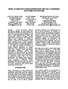
to use this measure in fault diagnosis on TE process [25]. TE process is a realistic simulation program of a chemical plant which has been widely studied as a benchmark in many PM-FD methods. In our paper, the data sets of TE process are downloaded from (http://depts.washington.edu/control/ LARRY/TE/download.html). In this database, there are 21 faults, named as IDV(1), IDV(2), . . . , IDV(21) (please refer to [24, 26] for more details). IDV(1–20) are process faults while IDV(21) is an additional value fault. There are 22 training sets and 22 testing sets in the database, including 21 faults measurement signals and one normal data set. 41 process variables and 11 manipulated variables consist of 52 measurement variables or features. Each training data file contains 480 rows which record the 52 measurement signals for 24 operation hours. Meanwhile, the data in each testing data set is collected via 48-hour plant operation time, in which the faults occur at the beginning of the 8th operation hour. That is to say, each testing data file contains 960 rows, while the first 160 rows represent the normal data and the following 800 points are abnormal data. The proposed fault diagnosis framework consists of 4 steps, that is, data preprocessing, metric learning, MTS pieces building, and MTS classification. First of all, all the measurement signals in training data and testing data are normalized in the data preprocessing. After that, we use the training data to learn a Mahalanobis distance. Then, the MTS pieces are built both in the training set and testing set. Finally, the testing MTS pieces are compared with training MTS pieces and we use KNN algorithm to determine the label (normal or abnormal) of the testing MTS pieces. In this paper, we assume that the normal measurement signals follow multivariate Gaussian distribution. In fault signals, some data but not all data are out of the confidence interval. The normal data is always in the obviously centralized distribution while abnormal data is lowly concentrated, even dispersive. There are two main problems when measuring the similarity between fault signals. The first one is that the amplitude between training data and testing data might be different. Figures 1(a) and 1(b) show the 46th measurement signals of IDV(0) and IDV(13). When considering the IDV(13), we can see that the amplitude of the testing data is obviously larger than that of training data. The second one is that the difference between abnormal signals may be larger than the difference between abnormal signals and normal signals. From Figures 1(e) and 1(f), we can see that some data of 19th measurement signal in the training data of IDV(21) is out of the upper limit of the confidence interval while some data in the testing data is out of the lower limit of confidence interval. This will result in two much false fault missing results. Therefore, an appropriate data preprocessing method should deal with these two problems at the same time. In our method, we apply the Gaussian kernel to normalize the original measurement signals. Consider 2

𝑥𝑖 (𝑡) = exp (−

(𝑥𝑖 (𝑡) − 𝜇𝑖 ) ), 2𝜎𝑖2

(10)

where 𝑥𝑖 (𝑡) represent the 𝑖th original measurement signal and 𝑥𝑖 (𝑡) is the normalized measurement signal. In this equation,

the parameters 𝜇𝑖 and 𝜎𝑖 are the mean value and variance evaluated using the 𝑖th normal measurement signal. Figures 1(c), 1(d), 1(g), and 1(h), respectively, show the normalized measurement signals of normal data set and fault data set. We can see that the normal signals concentrate near 1 while some data in fault signals is much less than 1. Besides, all large amplitude in the original fault signals will map to small value nearby 0 in the normalized signals and the difference between testing data and training data is very small. At the same time, the fault data which are out of the upper limit or lower limit of the confidence interval are almost the same in the normalized signals, which will be easy to measure their similarity. In our proposed multivariate dynamic time warping measure, how to learn an appropriate Mahalanobis distance is another key problem in our framework. Metric learning is a popular approach to accomplish such a learning process. In our previous work [27], we have proposed a Logdet divergence based metric learning (LDML) method to learn such a Mahalanobis distance function. After data processing, we use the normalized points in measurement signals to build 𝑖

𝑗

𝑘

𝑖

𝑗

the triplet labels {𝑋 , 𝑋 , 𝑋 }, which means that 𝑋 and 𝑋 𝑘 are in the same category while 𝑋 is in another category. The objective of metric learning is to ensure that most of the 𝑖

𝑗

𝑘

triplet labels {𝑋 , 𝑋 , 𝑋 } satisfy the fact that 𝑖

𝑗

𝑖

𝑘

𝑑𝑀 (𝑋 , 𝑋 ) − 𝑑𝑀 (𝑋 , 𝑋 ) ≤ −𝜌

(11)

while 𝜌 > 0. The updating formulation of the LDML algorithm is expressed as

Γ = 𝑀𝑡 −

𝑀𝑡+1 = Γ +

𝑖

𝑗

𝑖

𝑗 𝑇

𝑗 𝑇

𝑖

𝛼𝑀𝑡 (𝑋 − 𝑋 ) (𝑋 − 𝑋 ) 𝑀𝑡 𝑖

𝑗

1 + 𝛼(𝑋 − 𝑋 ) 𝑀𝑡 (𝑋 − 𝑋 ) 𝑖

𝑘

𝑖

𝑘 𝑇

, (12)

𝑘 𝑇

𝑖

𝛼𝑀𝑡 (𝑋 − 𝑋 ) (𝑋 − 𝑋 ) 𝑀𝑡 𝑖

𝑘

1 − 𝛼(𝑋 − 𝑋 ) 𝑀𝑡 (𝑋 − 𝑋 )

,

while 𝑀0 = 𝐼 and 𝛼 is the learning rate parameter (please refer to [27] for more details). This algorithm can accurately and robustly obtain the Mahalanobis distance which can distinguish fault and normal signals. From Figures 1(c) and 1(d), we can see that the integral trends of fault signal in training data and testing data do not match exactly. However, some pieces in the testing data can be found in the training data. Therefore, we use MTS pieces instead of the whole measurement signals in the following classification process. Each MTS piece contains 𝑎 continuous points in the training data or testing data. In the experiment, we have proven that when 𝑎 is selected as 12∼16, the proposed method will have the best performance. We measure the similarity between testing MTS pieces and all the training MTS pieces, including the normal data and fault data. Then, we use the KNN algorithm to classify MTS pieces as the normal ones or fault ones.


5

30

30

25

25

20

20

15

15

10

10 0

100

200

300

400

500

0

200

400

(a)

0

200

800

0

100

400

200

300

400

500

IDV(0) IDV(13)

IDV(0) Normal data in IDV(13) Abnormal data in IDV(13)

IDV(0) IDV(13)

1 0.9 0.8 0.7 0.6 0.5 0.4 0.3 0.2 0.1 0

600

1 0.9 0.8 0.7 0.6 0.5 0.4 0.3 0.2 0.1 0

(c)

(b)

600

280 270 260 250 240 230 220 210 200

800

280 260 240 220 200 180 0


100

200

400

500

160

0

200

(e)

0

100

200

300

400

500

IDV(0) IDV(21)

(g)

400

600

800


IDV(0) IDV(21)

(d)

1.05 1 0.95 0.9 0.85 0.8 0.75 0.7 0.65 0.6

300

(f)

1.05 1 0.95 0.9 0.85 0.8 0.75 0.7 0.65 0.6

0

200

400

600

800

IDV (0) Normal data in IDV(21) Abnormal data in IDV(21)

(h)

Figure 1: The comparison of original data and the data after preprocessing. (a)–(d) illustrate the comparison on the 46th measurement signals on IDV(0) and IDV(13): (a) original training data; (b) original testing data; (c) training data after preprocessing; (d) and testing data after preprocessing. (e)–(h) illustrate the comparison on the 19th measurement signals on IDV(0) and IDV(21): (e) original training data; (f) original testing data; (g) training data after preprocessing; (h) and testing data after preprocessing.

4. Experiments Results In this section, we conduct experiments on the TE process to illustrate the performance of the proposed fault diagnosis framework. In the following experiments, all experiments are tested in MATLAB 2011b, and all tests are implemented on a computer with Intel (R) Core (TM) i3-3120 M, 2.50 GHz CPU, 4 G RAM, and Windows 7 operating system. In this paper, we use two general indices to test the performance to evaluate PM-FD performance. They are fault detection rate (FDR)

and false alarm rate (FAR). Assume that 𝑡𝑝, 𝑡𝑛, 𝑓𝑝, and 𝑓𝑛, respectively, represent correct fault detection results, correct normal signal detection results, false fault alarm results, and false fault missing results. The definitions of these FDR and FAR are given as 𝑡𝑝 × 100%, FDR = 𝑡𝑝 + 𝑓𝑛 (13) 𝑓𝑝 FAR = × 100%. 𝑓𝑝 + 𝑡𝑛

Abstract and Applied Analysis 100

100

90

95

80

90

Fault detection rate (%)

Fault detection rate (%)

6

70 60 50 40

80 75 70 65

30 20

85

0

5

10 15 20 Fault alarm rate (%)

25

30

20 points EER

10 points 12 points 16 points (a)

60

5

0

10 Fault alarm rate (%)

15

20

20 points EER

10 points 12 points 16 points (b)

Figure 2: The relationship between the fault diagnosis performance and the length of the MTS pieces. The points on FAR-FDR curves record the experimental results with different 𝑘 in KNN algorithm. Among these points, the one which is the closest to the EER curve represents the fault diagnosis performance. The experimental results reveal that the proposed method will have the best performance when the length of the MTS pieces is set as 16. (a) The results on IDV(11). (b) The results on IDV(21).

Another important performance index is chosen as equal error rate (EER), where the FAR and false fault missing rate (1−FDR) are equal to each other. As mentioned above, in our algorithm, the PM-FD process is regarded as a classification problem. In the KNN classification algorithm, different 𝑘 will produce different FDR and FAR. In our experiment, the performance is chosen as the FDR and FAR which is the closest to the EER line. The first experiment is to illustrate the relationship between the fault diagnosis performance and the length of the MTS pieces. We, respectively, use MTS pieces with 10, 12, 16, and 20 points to separately detect the IDV(11) and IDV(21). The experimental results with different 𝑘 are illustrated in Figure 2. From the results, we can see that the FDR rises when the length of MTS pieces increases from 10 points to 16 points. However, when the length of MTS pieces rises to 20 points, the performance will degrade. The reason for the phenomena can be explained as follows. When the length of MTS pieces is too short, these MTS contain too little information to record the trends and variation of the measurement signals completely. The comparison of MTS will be inaccurate and the performance will degrade. In an extreme case, the length of MTS pieces is 1 and the algorithm degrades to the traditional methods which are based on measuring the similarity of static feature points. If the length of MTS pieces is too long, it will tend to measure the integral similarity of signals. As mentioned above, in some measurement signals, the integral trends can not match each other, but some pieces in the testing data are similar to those in the training data. Thus, the performance will also have

a risk of declining. The experimental results suggest that the best length of the MTS pieces is 12∼16. In the second experiment, we compare the proposed method with many other classical PM-FD methods, including PCA, DPCA, ICA, MICA, FDA, PLS, TPLS, MPLS, and SAP. The results of the proposed method are average values over 5 runs while the results of other classical PMFD methods are reported by literature [26]. The testing results of various methods for all data sets are summarized in Table 1. The first 21 rows record the FDR for all the faults. Inspired by the literature [26], we also classified 21 faults as three categories. The first category consists of IDV(1-2), IDV(4–8), IDV(12–14), and IDV(17-18). These faults can be easily detected by all the methods. Almost all the methods have high FDR as well as low FAR in the fault diagnosing process. The faults in the second category, including IDV(1011), IDV(16), IDV(19) and IDV(20-21), are not easy to detect. And the performance of methods on these faults will have obvious difference. In the last category, all methods perform bad results because these faults are very hard to detect. The last row illustrates the average FAR by detecting faults on the fault-free signals of IDV(0). From the results, we can see that the proposed method has good performance on most of the faults in the first and third categories. At the same time, the performance of the proposed method is not bad on the rest of faults, such as IDV(10–12), IDV(16), and IDV(20). Our method does not perform well on IDV(5) and IDV(19). The reasons can be explained as follows. The measurement signals of IDV(5) have obvious difference when the fault occurs. However, the IDV(5) and normal signals have almost the same trend after a certain time, which can


7

Table 1: FDRs (%) and FARs (%) comparison with classical PM-FD methods on TE data sets given in [24]. Fault (free) IDV(1) IDV(2) IDV(4) IDV(5) IDV(6) IDV(7) IDV(8) IDV(12) IDV(13) IDV(14) IDV(17) IDV(18) IDV(10) IDV(11) IDV(16) IDV(19) IDV(20) IDV(21) IDV(3) IDV(9) IDV(15) IDV(0)

PCA 99.88 98.75 100 33.63 100 100 98.00 99.13 95.38 100 95.25 90.50 60.50 78.88 55.25 41.13 63.38 52.13 12.88 8.38 14.13 6.13

DPCA 99.88 99.38 100 43.25 100 100 98.00 99.25 95.38 100 97.25 90.88 72.00 91.50 67.38 87.25 73.75 61.00 12.25 12.88 19.75 10.13

ICA 100 98.25 100 100 100 100 98.25 99.88 95.25 100 96.88 90.50 89.25 78.88 92.38 92.38 91.38 56.38 4.50 4.75 7.75 2.75

MICA 99.88 98.25 87.63 100 100 100 97.63 99.88 95.00 99.88 93.00 89.75 85.88 61.63 83.38 80.25 86.00 70.75 14.25 8.88 10.75 1.63

not be detected by the proposed method. On the contrary, the measurement signals of IDV(19) are similar to normal signals at the beginning and then the difference became noticeable after a period of running time. Our method is not good at detecting this kind of fault too.

5. Conclusion In this paper, we propose a novel framework for data-driven PM-FD problems. One contribution of this paper is that it firstly uses MTS pieces to represent the measurement signals as dynamic features in the measurement signals can provide more information than static features. Besides, this paper uses a Mahalanobis distance based DTW algorithm to measure the difference between two MTS. The method can build an accurate relationship between the variables and the labels of the signals, which is a benefit for the classification of measurement signals. Furthermore, we also present a new PM-FD framework which is based on Mahalanobis distance based DTW algorithm. The proposed algorithm is shown to be precise by experiments on benchmark data sets and comparison with classical PM-FD methods. One drawback of this algorithm is the heavy time consumption in measuring the similarity of MTS. In future, we will concentrate on further optimization of the proposed method with respect to computation efficiency and other issues.

Conflict of Interests The authors declare that there is no conflict of interests regarding the publication of this paper.

FDA 100 98.75 100 100 100 100 98.13 99.75 95.63 100 96.63 90.75 87.13 73.38 83.25 87.88 81.88 52.75 7.00 6.25 12.63 6.38

PLS 99.88 98.63 99.50 33.63 100 100 97.88 99.25 95.25 100 94.25 90.75 82.63 78.63 68.38 26.00 62.75 59.88 14.25 14.50 23.00 10

TPLS 99.88 98.88 100 100 100 100 98.50 99.63 96.13 100 96.00 91.88 91.00 86.13 90.75 82.88 78.38 66.38 24.25 23.50 29.88 19.62

MPLS 100 98.88 100 100 100 100 98.63 99.88 95.50 100 97.13 91.25 91.13 83.25 94.28 94.25 91.50 72.75 18.75 12.13 23.25 10.75

SAP 99.63 97.88 99.88 100 100 99.88 95.88 99.88 94.88 97.63 97.13 91.00 95.50 84.75 94.88 88.50 83.75 38.63 6.38 0.88 29.50 1.5

Proposed 100 100 100 89.47 100 100 100 99.15 96.61 100 98.48 94.87 83.54 89.47 83.67 77.55 84.21 89.39 35.90 48.72 38.46 3.32

Acknowledgment The research leading to these results has received funding from the Polish-Norwegian Research Programme operated by the National Centre for Research and 24 Development under the Norwegian Financial Mechanism 2009–2014 in the frame of Project Contract no. Pol-Nor/200957/47/2013.

References [1] S. Yin, X. Yang, and H. R. Karimi, “Data-driven adaptive observer for fault diagnosis,” Mathematical Problems in Engineering, vol. 2012, Article ID 832836, 21 pages, 2012. [2] S. Yin, S. X. Ding, A. H. A. Sari, and H. Hao, “Data-driven monitoring for stochastic systems and its application on batch process,” International Journal of Systems Science, vol. 44, no. 7, pp. 1366–1376, 2013. [3] V. Venkatasubramanian, R. Rengaswamy, K. Yin, and S. N. Kavuri, “A review of process fault detection and diagnosis part I: quantitative model-based methods,” Computers and Chemical Engineering, vol. 27, no. 3, pp. 293–311, 2003. [4] W. Chen and M. Saif, “Observer-based fault diagnosis of satellite systems subject to time-varying thruster faults,” Journal of Dynamic Systems, Measurement and Control, Transactions of the ASME, vol. 129, no. 3, pp. 352–356, 2007. [5] P. Zhang, H. Ye, S. X. Ding, G. Z. Wang, and D. H. Zhou, “On the relationship between parity space and H2 approaches to fault detection,” Systems and Control Letters, vol. 55, no. 2, pp. 94–100, 2006. [6] J. Suonan and J. Qi, “An accurate fault location algorithm for transmission line based on R-L model parameter identification,” Electric Power Systems Research, vol. 76, no. 1–3, pp. 17–24, 2005.

8 [7] M. A. Schwabacher, “A survey of data-driven prognostics,” in Proceedings of the Advancing Contemporary Aerospace Technologies and Their Integration (InfoTech ’05), pp. 887–891, September 2005. [8] S. Yin, G. Wang, and H. R. Karimi, “Data-driven design of robust fault detection system for wind turbines,” Mechatronics. In press. [9] S. Yin, H. Luo, and S. Ding, “Real-time implementation of faulttolerant control systems with performance optimization,” IEEE Transactions on Industrial Electronics, vol. 61, no. 5, pp. 2402– 2411, 2012. [10] L. H. Chiang, E. L. Russell, and R. D. Braatz, “Fault diagnosis in chemical processes using Fisher discriminant analysis, discriminant partial least squares, and principal component analysis,” Chemometrics and Intelligent Laboratory Systems, vol. 50, no. 2, pp. 243–252, 2000. [11] M. Misra, H. H. Yue, S. J. Qin, and C. Ling, “Multivariate process monitoring and fault diagnosis by multi-scale PCA,” Computers and Chemical Engineering, vol. 26, no. 9, pp. 1281–1293, 2002. [12] S. Ding, P. Zhang, E. Ding et al., “On the application of PCA technique to fault diagnosis,” Tsinghua Science and Technology, vol. 15, no. 2, pp. 138–144, 2010. [13] W. Ku, R. H. Storer, and C. Georgakis, “Disturbance detection and isolation by dynamic principal component analysis,” Chemometrics and Intelligent Laboratory Systems, vol. 30, no. 1, pp. 179–196, 1995. [14] Y. Zhang, H. Zhou, S. J. Qin, and T. Chai, “Decentralized fault diagnosis of large-scale processes using multiblock kernel partial least squares,” IEEE Transactions on Industrial Informatics, vol. 6, no. 1, pp. 3–10, 2010. [15] M. R. Maurya, R. Rengaswamy, and V. Venkatasubramanian, “Fault diagnosis using dynamic trend analysis: a review and recent developments,” Engineering Applications of Artificial Intelligence, vol. 20, no. 2, pp. 133–146, 2007. [16] S. Yin, S. X. Ding, P. Zhang, A. Hagahni, and A. Naik, “Study on modifications of pls approach for process monitoring,” Threshold, vol. 2, pp. 12389–12394, 2011. [17] M. Kano, S. Tanaka, S. Hasebe, I. Hashimoto, and H. Ohno, “Monitoring independent components for fault detection,” AIChE Journal, vol. 49, no. 4, pp. 969–976, 2003. [18] J.-M. Lee, S. J. Qin, and I.-B. Lee, “Fault detection and diagnosis based on modified independent component analysis,” AIChE Journal, vol. 52, no. 10, pp. 3501–3514, 2006. [19] Q. P. He, S. J. Qin, and J. Wang, “A new fault diagnosis method using fault directions in Fisher discriminant analysis,” AIChE Journal, vol. 51, no. 2, pp. 555–571, 2005. [20] S. X. Ding, P. Zhang, A. Naik, E. L. Ding, and B. Huang, “Subspace method aided data-driven design of fault detection and isolation systems,” Journal of Process Control, vol. 19, no. 9, pp. 1496–1510, 2009. [21] T. G. Holt, M. Reinders, and E. Hendriks, “Multi-dimensional dynamic time warping for gesture recognition,” in Proceedings of the 13th Annual Conference of the Advanced School for Computing and Imaging, vol. 119, 2007. [22] S. Salvador and P. Chan, “Toward accurate dynamic time warping in linear time and space,” Intelligent Data Analysis, vol. 11, no. 5, pp. 561–580, 2007. [23] G. Al-Naymat, S. Chawla, and J. Taheri, “Sparsedtw: a novel approach to speed up dynamic time warping,” in Proceedings of the 8th Australasian Data Mining Conference, vol. 101, Computer Society, Australian, 2009.

Abstract and Applied Analysis [24] L. H. Chiang, R. D. Braatz, and E. L. Russell, Fault Detection and Diagnosis in Industrial Systems, Springer, 2001. [25] J. J. Downs and E. F. Vogel, “A plant-wide industrial process control problem,” Computers and Chemical Engineering, vol. 17, no. 3, pp. 245–255, 1993. [26] S. Yin, S. X. Ding, A. Haghani, H. Hao, and P. Zhang, “A comparison study of basic data-driven fault diagnosis and process monitoring methods on the benchmark tennessee eastman process,” Journal of Process Control, vol. 22, no. 9, pp. 1567–1581, 2012. [27] J. Mei, M. Liu, H. R. Karimi, and H. Gao, Logdet Divergence Based Metric Learning Using Triplet Labels, ICML Workshop on Divergences.

Advances in

Operations Research Hindawi Publishing Corporation http://www.hindawi.com

Volume 2014

Advances in

Decision Sciences Hindawi Publishing Corporation http://www.hindawi.com

Volume 2014

Journal of

Applied Mathematics

Algebra

Hindawi Publishing Corporation http://www.hindawi.com


Volume 2014

Journal of

Probability and Statistics Volume 2014

The Scientific World Journal Hindawi Publishing Corporation http://www.hindawi.com


Volume 2014

International Journal of

Differential Equations Hindawi Publishing Corporation http://www.hindawi.com

Volume 2014

Volume 2014

Submit your manuscripts at http://www.hindawi.com International Journal of

Advances in

Combinatorics Hindawi Publishing Corporation http://www.hindawi.com

Mathematical Physics Hindawi Publishing Corporation http://www.hindawi.com

Volume 2014

Journal of

Complex Analysis Hindawi Publishing Corporation http://www.hindawi.com

Volume 2014

International Journal of Mathematics and Mathematical Sciences

Mathematical Problems in Engineering

Journal of

Mathematics Hindawi Publishing Corporation http://www.hindawi.com

Volume 2014


Volume 2014

Volume 2014


Volume 2014

Discrete Mathematics

Journal of

Volume 2014


Discrete Dynamics in Nature and Society

Journal of

Function Spaces Hindawi Publishing Corporation http://www.hindawi.com


Volume 2014


Volume 2014


Volume 2014

International Journal of

Journal of

Stochastic Analysis

Optimization



Volume 2014

Volume 2014