A Novel Density Peak Clustering Algorithm based on Squared Residual Error Milan Parmar†‡ , Di Wang§ , Ah-Hwee Tan§¶ , Chunyan Miao§¶ , Jianhua Jiang‡ , You Zhou†∗ † College
of Computer Science and Technology Jilin University Changchun, China ‡ School of Management Science and Information Engineering Jilin University of Finance and Economics Changchun, China § Joint NTU-UBC Research Centre of Excellence in Active Living for the Elderly ¶ School of Computer Science and Engineering Nanyang Technological University Singapore ∗ Corresponding Author
[email protected], {wangdi, asahtan, ascymiao}@ntu.edu.sg,
[email protected],
[email protected] Abstract—The density peak clustering (DPC) algorithm is designed to quickly identify intricate-shaped clusters with high dimensionality by finding high-density peaks in a non-iterative manner and using only one threshold parameter. However, DPC has certain limitations in processing low-density data points because it only takes the global data density distribution into account. As such, DPC may confine in forming low-density data clusters, or in other words, DPC may fail in detecting anomalies and borderline points. In this paper, we analyze the limitations of DPC and propose a novel density peak clustering algorithm to better handle low-density clustering tasks. Specifically, our algorithm provides a better decision graph comparing to DPC for the determination of cluster centroids. Experimental results show that our algorithm outperforms DPC and other clustering algorithms on the benchmarking datasets. Index Terms—clustering, density peak clustering, squared residual error, low-density data points
I. I NTRODUCTION Clustering algorithms aim to analyze data by discovering their underlying structure and organize them into separate categories according to their characteristics expressed as internal homogeneity and external bifurcation without prioriknowledge. Successful applications of clustering techniques are evident in various domains, such as pattern recognition [1] [2], bioinformatics [3], disease diagnosis [4], risk analysis [5] [6], etc. Moreover, some emerging topics such as big data [7], virtual reality [8], IoT [9], etc., also avail from clustering methods. In general, clustering methods can be broadly categorized into five groups based on their dynamics: partitioning [10], hierarchical [11] [12], density-based [13], model-based [14], and grid-based [15]. This research is supported in part by the Science & Technology Development Foundation of Jilin Province under grant No. 20160101259JC and the National Science Fund Project of China No. 61772227. This research is also supported in part by the National Research Foundation, Prime Minister’s Office, Singapore under its IDM Futures Funding Initiative.
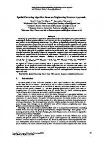
Density-based clustering methods have been widely used to form arbitrary shape clusters by detecting high-density regions in the high dimensional data space. Fundamentally, the region with high density, or a set of densely connected data points, in the data space is treated as a cluster. Densitybased spatial clustering of applications with noise (DBSCAN) [16] is probably the most well-known density-based clustering algorithm engendered from the basic notion of the local density, which creates arbitrary-shaped clusters. Recently, densitybased clustering methods have attracted more attention since Rodriguez and Liao proposed their density peak clustering (DPC) algorithm [17] in 2014. The desirable features of DPC include detection of non-spherical clusters without specifying the number of clusters, few number of control parameters, and autonomous identification of cluster centroids for varying cluster sizes and within-cluster density. However, DPC has its limitations. Alike DBSCAN, DPC may fail to capture thin clusters by using its decision graph (see Section II), i.e., it does not perform well on anomaly detection. Data distribution within clusters has to be carefully examined to detect anomalies, mainly because the presence of anomalies is a clear sign of erroneous conditions that may lead to significant performance degradation [18]. As shown in Fig. 1, DPC generates groups of data points by identifying clusters with maximum density, but does not handle well the uneven distribution in individual clusters (also pointed out in [19]), e.g., the two anomalies (at top left corner) are always considered as part of a larger cluster regardless of different Cd values, where Cd denotes the user specified cutoff disctance (see Section II). In such cases, it is difficult for DPC to pick up all the outliers with varying Cd values and it may not be able to find clusters of small sizes or consisting of borderline points and outliers (relatively speaking) only. Furthermore, when the dimensionality of the underlying dataset increases, the well-known “curse of dimensionality” problem [20] will
28
28
26
26
24
24
22
22
20
20
18
18
16
14
The rest of the paper is organized as follows. We briefly introduce the dynamics of DPC in Section II. We present our proposed clustering method based on squared residual error in Section III. We report the experimental results with comparisons and discussions in Section IV. We draw the conclusion and propose future work in Section V.
16
0
5
10
15
14
0
5
10
15
II. R ELATED W ORK (a) Cd = 0.9301
(b) Cd = 1.3124
28
28
26
26
24
24
22
22
20
20
18
18
16
14
16
0
5
10
(c) Cd = 2.1213
15
14
0
5
10
15
(d) Cd = 3.2381
Fig. 1. Visualizations of clusters identified in the Flame dataset by DPC with different Cd parameter values.
exacerbate. Hence, in this paper, we propose a novel densitybased clustering algorithm to detect anomalies that cannot be identified using existing methods. As a result, the proposed algorithm can better identify and handle various types of anomalies manifested in different patterns. To correctly and efficiently identify the anomalies and consequently finalize the cluster formation, we rely on using the concept of halo points to unravel low-density points in the following two ways (see Section III-C for more technical details): (i) halo points identification: a set of low-density points are considered as halo points, and (ii) halo points decision: halo points can be categorized into outliers and borderline points that they are either merged into certain existing clusters or used to form new clusters. To better deal with halo points and hence increase the clustering performance, in this paper, we propose an effective density-based clustering algorithm based on squared residual error (e2 ) [21]. The main contributions of our proposed clustering method are listed as follows:
We present the dynamics, pros and cons of DPC in this literature review section. In a nutshell, DPC generates clusters by assigning data points to the same cluster of its nearest neighbor with higher density. Moreover, DPC uses the decision graph approach to identify cluster centroids. A decision graph is derived based on the following two fundamental properties of each data point xi : (i) local density ρi and (ii) individual distance of each data point from points of higher density δi . Assume a dataset consists of XP ×M = [x1 , x2 , ..., xP ]T , where xi = [x1i , x2i , ..., xM i ] is a vector with M attributes and P is the total number of data points. The distance between two data points xi and xj is computed as follows: dij = || xi − xj ||.
(1)
The local density of a data point xi , denoted as ρi and known as the hard threshold [17], is then defined as: ρi =
X
χ(x) · (dij − Cd ),
(2)
j
where χ(x) = 1, if x < 0, and Cd is the cutoff distance that user specified to control the weight degradation rate. The determination of Cd is actually the assignment of the average number of neighbors that each data point has. Specifically, ρi is defined as the number of data points that have shorter distance than Cd and are adjacent to xi . Another way of local density computation known as the soft threshold [17] is defined as follows: ! X dij2 (3) ρi = exp − 2 . Cd j
1) We incorporate the squared residual error theory to enable the discovery of anomalies and borderline points by identifying the halo points. 2) The decision graph derived by our proposed clustering method can better identify the cluster centroids and aggregate clusters. 3) Halo points make it easier to isolate anomalies from borderline points.
δi is defined as the shortest distance from any other data point that has a higher density value than xi . If xi has the highest density value, δi is assigned to the longest distance to any other data point. Specifically, δi is computed as follows: if ∃ j s.t. ρj > ρi, min dij, j:ρj >ρi δi = (4) max dij, otherwise.
We apply our proposed algorithm on four synthetic datasets and four UCI datasets for performance evaluations. We also apply K-Means [22], affinity propagation (AP) [11] and DPC on the same datasets for comparisons. Experimental results show that our algorithm achieves the best performance on most datasets (specifically, best on seven out of eight datasets and the second best on the remaining dataset).
DPC finds a border region for each cluster, where the region is defined as the set of points assigned to that cluster but within certain distance (i.e., Cd ) from the data points belonging to another cluster. Subsequently, DPC finds the data point of the highest density within the border region of that cluster and denotes its density as ρb . The data points of the cluster whose density is higher than ρb are considered as part of the
j
data point xi to its neighbor xj is determined by the distance between xi and xj and the neighborhood size:
1.5
7 1 6
1
5
0.5
4
e2ij =
δ
0
3 2 -0.5
2 1
-1
0
-1.5 -4
0
5
10
15
20
-3
-2
-1
0
1
2
3
4
ρ
(a) Iris decision graph by DPC
(b) Iris cluster formation by DPC
Fig. 2. Determination of cluster centroids and the resulting cluster formation based on the decision graph generated by DPC on the Iris dataset.
cluster core and others are considered as part of the cluster halo (suitable to be considered as noise) [17]. The performance of DPC is highly sensitive to the identification of the cluster centroids [17]. Cluster centroids with high local density ρ and high δ can be easily identified in the decision graph (see Fig. 2(a)). Nevertheless, it is difficult for DPC to identify cluster centroids with low ρ and high δ, or with high ρ and low δ. III. REDPC: R ESIDUAL E RROR - BASED D ENSITY P EAK C LUSTERING A LGORITHM In this section, we present our proposed clustering algorithm named Residual Error-based Density Peak Clustering (REDPC), which inherits the strengths of centroid detection from DPC [17], distance measure from residual error theory [21], and density-connectivity from DBSCAN [16]. The dynamics of REDPC are designed according to the following two bases: 1) A cluster is formed when its centroid is surrounded by only the data points with higher residual error. 2) A data point can be assigned to the cluster when there is another data point with higher δ (see the following subsection) and lower residual error. The overall REDPC procedure consists of the following four stages and each stage is elaborated in the following subsections, respectively. 1) Preprocessing: compute the squared residual error between data points and compute δ. 2) Initial assignments: generate the decision graph based on residual errors, identify centroids, and assign data points with their respective cluster label. 3) Halo identification: identify halo points (consists of borderline points and anomalies). 4) Final refinements: detect and isolate anomalies from halo points and output the final clustering results (with anomalies represented using special symbols). A. Preprocessing Unlike DPC [17], we incorporate the residual error approach instead of relying on local density between data points, because residual error constructs a more informative decision graph in the later stage, which may lead to better clustering performance. Specifically, the squared residual error (e2ij ) of a
|| xi − xj || | Ni |
2
2
,
(5)
where || · || denotes Euclidean distance, N is a predefined parameter, which defines the neighborhood size, and | Ni | denotes the number of data points in Ni . Similar to DPC, a cut-off residual Cd value is predefined and later in Section III-C, Cd is used to identify halo points. δi denotes the minimum distance of data point xi to another data point with lower residual error. δi is computed as follows:
δi =
|| xi − xj ||, j:(emin 2 ) 1 border e2 ← ones(1, Total(X)) for i ← 1:n-1 do for j ← i+1:n do if Cl(i) ∼ = Cl(j) && DM(i, j) border e2 (Cl(i)) then halo(i)← 0 (halo point identified not belong to any class (0)) end if end if haloset = find(halo(:)==0) % put all halo points in haloset
D. Final Refinements During anomaly detection, a halo point with high residual error and high δ (these threshold values are auto-derived, see Algorithm 3) is recognized as an anomaly. All the anomalies are collected in the anoset. The final clustering results are then
Algorithm 3 Anomaly identification. Require: haloset (vector of halo points) Ensure: anoset (vector of anomalies points) Set thresold limit for e2 and δ for anomaly detection limit e2 ← mean(e2 )+ sortd(e2 )*0.8 limit δ ← max(δ)+min(δ)/2 for i ← 1:haloset do % for every halo point if Cl(i) > limit e2 && δi < limit δ then ano(i) ← 0 % anomaly identified end if end for anoset = find(ano(:)==0) % put all anomalies in anoset It is of great importance to distinguish the anomalies from normal data points and reasonable outliers because anomalies highly likely represent the abnormal patterns or malicious activities in real-world scenarios. For example, unusual road traffic patterns may suggest nearby accidents or emergencies, unusual credit card transactions may indicate identity theft, unusual computer network loads should alert the cyber security division, etc. IV. E XPERIMENTAL R ESULTS To test the feasibility and validate the robustness of REDPC, we compare its performance with K-Means [22], AP [11], and DPC [17] on three widely-used synthetic clustering datasets, namely Flame, Aggression and Spiral, four UCI datasets, namely Iris, Seeds, Wine and Glass, and one own-defined dataset D21 . The properties of all eight datasets are listed in Table I. In this paper, we use F -score to measure the accuracy of the clustering results. The performance comparisons among all the benchmarking models are reported in Table II. It is encouraging to find that REDPC achieves the highest F -score on seven out of eight datasets. Although REDPC only achieves the second best on Seed, the difference between the winner is as small as 0.8068 − 0.8065 = 0.0003 or 0.03%. 1 The D2 dataset (with cluster labels) is available online: https://www. dropbox.com/s/899xltgq3gg09bg/D2 with label.csv?dl=0
TABLE II F - SCORE ON EIGHT BENCHMARKING DATASETS Dataset Iris Seeds Wine Glass Spiral Flame Aggregation D2
K-Means 0.8208 0.8068 0.5835 0.5052 0.3277 0.7364 0.7725 0.4333
AP 0.4851 0.3877 0.3142 0.2874 0.2853 0.2874 0.3429 0.4332
DPC 0.7715 0.8026 0.5892 0.5418 1 1 1 1
REDPC 0.8404 0.8065 0.5892 0.5542 1 1 1 1
28
28
26
26
24
24
22
22
20
20
18
18
16
16
14
14 0
5
10
0
15
(a) K-Means, K = 3
5
10
15
(b) AP, preference = -5.9261
28
28
26
26
24
24
22
22
20
20
18
18
16
16
4.5
7 10 1 6
4 5 3.5
δ
4
3
97 2
3
14
14 0
2
1
0 0
121 3 102 76 129 94126 106 81 109 135 136 53 116 69 115 63 139 1 92 117 131 23 120 65 101 15 137 103 60 86 148 84 45 6199 113 6 17 112 33 34 80 7273 134 19 56 52 77 122 78 48 39 32 37 67 62 105 125 25 87 150 21 93 141 75 91 51 57 108130 123 8816 90 127 59 104 68 145 5146 5114 14 147 142 149 49 2 795 12 766 36 44 144 71 74 111 26 43 79 98 24 54 85 89 70 124 140 4028 29 13 541 30 50 420 100 46 96 22 347 128 83 64 9 82 138 58 8231 11 133 35 18 38 143 0.1 0.2 0.3 0.4 0.5
5
10
15
0
5
10
15
2.5 110 42 119
118 107 132
(c) DPC, Cd = 1.6008
2 0.6
0.7
4
4.5
5
5.5
6
6.5
7
7.5
(d) REDPC, Ni = 5, Cd = 1.4577 (#clusters = 2, #anomalies = 2)
8
e2
(a) Iris decision graph by REDPC
(b) Cluster formation by REDPC
Fig. 4. Determination of cluster centroids and the resulting cluster formation based on the decision graph generated by REDPC on the Iris dataset.
Other than REDPC always performs better or equally good when compared to DPC, we find that it is much easier to identify cluster centroids by using the decision graph derived by REDPC than that by DPC. It is shown in Fig. 2(a) that the third cluster centroid is difficult to be identified merely based on ρ and δ. However, as shown in Fig. 4(a), the identification of the third cluster centroid is easier based on e2 and δ. More importantly, DPC does not perform well when there are ascertaining anomalies whose distance to higher density points is less than Cd . On the other hand, REDPC uses e2 as one of the identification criteria, which reduces the dependency of Cd . This is the main reason why REDPC outperforms DPC on all the UCI datasets. To illustrate the capability of REDPC in anomaly detection, we present the clustering results of applying all the benchmarking clustering methods on the Flame dataset in Fig. 5. Comparing Fig. 5(d) to the rest of the subfigures, it is clearly shown that only REDPC successfully identifies the anomalous data points in the top left corner (although both DPC and REDPC achieve 100% F -score). To illustrate the performance of REDPC on datasets with different density distributions, we present the clustering results of applying all the benchmarking clustering methods on the Aggregation dataset in Fig. 6. Fig. 6(d) shows that REDPC can perfectly handle clusters of different sizes with boundaries in close proximity. V. C ONCLUSION In this paper, we propose a novel density peak type of clustering method named REDPC by using squared residual error to better identify cluster centroids. The experimental results on both synthetic and real-world UCI datasets demonstrate that REDPC outperforms DPC and other clustering algorithms.
Fig. 5. An illustration of anomaly detection on the Flame dataset.
30
30
25
25
20
20
15
15
10
10
5
5
0
0 0
5
10
15
20
25
30
35
40
(a) K-Means, K = 7
0
5
10
15
20
25
30
35
40
(b) AP, preference = -16.5170
30
30
25
25
20
20
15
15
10
10
5
5
0
0 0
5
10
15
20
25
30
35
(c) DPC, Cd = 2.3162
40
0
5
10
15
20
25
30
35
40
(d) REDPC, Ni = 5, Cd = 1.8601
Fig. 6. Cluster formation on the Aggregation dataset.
Going forward, we will improve the proposed clustering algorithm for more autonomy in parameter value determinations, refinement in the clustering dynamics for better performance, and applications on more complex and challenging datasets. R EFERENCES [1] Z. Li, J. Liu, Y. Yang, X. Zhou, and H. Lu, “Clustering-guided sparse structural learning for unsupervised feature selection,” IEEE Transactions on Knowledge and Data Engineering, vol. 26, no. 9, pp. 2138– 2150, 2014. [2] J. Wen, D. Zhang, Y. Cheung, H. Liu, and X. You, “A batch rival penalized expectation-maximization algorithm for gaussian mixture clustering with automatic model selection.” Computational and Mathematical Methods in Medicine, vol. 2012, p. 425730, 2012. [3] C. Xu and Z. Su, “Identification of cell types from single-cell transcriptomes using a novel clustering method,” Bioinformatics, vol. 31, no. 12, pp. 1974–1980, 2015.
[4] D. Wang, C. Quek, and G. S. Ng, “Ovarian cancer diagnosis using a hybrid intelligent system with simple yet convincing rules,” Applied Soft Computing, vol. 20, pp. 25–39, 2014. [5] G. Kou, Y. Peng, and G. Wang, “Evaluation of clustering algorithms for financial risk analysis using MCDM methods,” Information Sciences, vol. 275, pp. 1–12, 2014. [6] D. Wang, C. Quek, and G. S. Ng, “Bank failure prediction using an accurate and interpretable neural fuzzy inference system,” AI Communications, vol. 29, no. 4, pp. 477–495, 2016. [7] A. Fahad, N. Alshatri, Z. Tari, A. Alamri, I. Khalil, A. Y. Zomaya, S. Foufou, and A. Bouras, “A survey of clustering algorithms for big data: Taxonomy and empirical analysis,” IEEE Transactions on Emerging Topics in Computing, vol. 2, no. 3, pp. 267–279, 2014. [8] A. Chaudhary, J. L. Raheja, K. Das, and S. Raheja, “Intelligent approaches to interact with machines using hand gesture recognition in natural way: A survey,” arXiv preprint arXiv:1303.2292, 2013. [9] C.-W. Tsai, C.-F. Lai, M.-C. Chiang, L. T. Yang et al., “Data mining for internet of things: A survey.” IEEE Communications Surveys and Tutorials, vol. 16, no. 1, pp. 77–97, 2014. [10] A. Mukhopadhyay, U. Maulik, S. Bandyopadhyay, and C. A. C. Coello, “Survey of multiobjective evolutionary algorithms for data mining: Part II,” IEEE Transactions on Evolutionary Computation, vol. 18, no. 1, pp. 20–35, 2014. [11] B. J. Frey and D. Dueck, “Clustering by passing messages between data points,” Science, vol. 315, no. 5814, pp. 972–976, 2007. [12] D. Wang and A.-H. Tan, “Self-regulated incremental clustering with focused preferences,” in Proceedings of International Joint Conference on Neural Networks. IEEE, 2016, pp. 1297–1304. [13] R. Mehmood, G. Zhang, R. Bie, H. Dawood, and H. Ahmad, “Clustering by fast search and find of density peaks via heat diffusion,” Neurocomputing, vol. 208, pp. 210–217, 2016. [14] T. Chen, N. L. Zhang, T. Liu, K. M. Poon, and Y. Wang, “Model-based multidimensional clustering of categorical data,” Artificial Intelligence, vol. 176, no. 1, pp. 2246–2269, 2012. [15] M. Parikh and T. Varma, “Survey on different grid based clustering algorithms,” International Journal of Advance Research in Computer Science and Management Studies, vol. 2, no. 2, 2014. [16] M. Ester, H.-P. Kriegel, J. Sander, and X. Xu, “A density-based algorithm for discovering clusters in large spatial databases with noise,” in Proceedings of International Conference on Knowledge Discovery and Data Mining, 1996, pp. 226–231. [17] A. Rodriguez and A. Laio, “Clustering by fast search and find of density peaks,” Science, vol. 344, no. 6191, pp. 1492–1496, 2014. [18] V. Chandola, A. Banerjee, and V. Kumar, “Anomaly detection: A survey,” ACM Computing Surveys, vol. 41, no. 3, p. 15, 2009. [19] M. Wang, W. Zuo, and Y. Wang, “An improved density peaks-based clustering method for social circle discovery in social networks,” Neurocomputing, vol. 179, pp. 219–227, 2016. [20] L. Parsons, E. Haque, and H. Liu, “Subspace clustering for high dimensional data: A review,” ACM SIGKDD Explorations Newsletter, vol. 6, no. 1, pp. 90–105, 2004. [21] H. Chang and D.-Y. Yeung, “Robust path-based spectral clustering,” Pattern Recognition, vol. 41, no. 1, pp. 191–203, 2008. [22] J. A. Hartigan and M. A. Wong, “Algorithm as 136: A k-means clustering algorithm,” Journal of the Royal Statistical Society. Series C (Applied Statistics), vol. 28, no. 1, pp. 100–108, 1979.