A Novel Dynamic Programming Algorithm for Track ... - IEEE Xplore

2608

IEEE TRANSACTIONS ON SIGNAL PROCESSING, VOL. 61, NO. 10, MAY 15, 2013

A Novel Dynamic Programming Algorithm for Track-Before-Detect in Radar Systems Emanuele Grossi, Member, IEEE, Marco Lops, Senior Member, IEEE, and Luca Venturino, Member, IEEE

Abstract—In this paper we present a novel procedure for multi-frame detection in radar systems. The proposed architecture consists of a pre-processing stage, which extracts a set of candidate alarms (or plots) from the raw data measurements (e.g., this can be the Detector and Plot-Extractor of common radar systems), and a track-before-detect (TBD) processor, which jointly elaborates observations from multiple scans (or frames) and confirms reliable plots. A computationally efficient dynamic programming algorithm for the TBD processor is derived, which does not require a discretization of the state space and operates directly on the input plot-lists. Finally, a simple algorithm to solve possible data association problems arising at the track-formation step is given, and a thorough complexity and performance analysis is provided, showing that large detection gains with respect to the standard radar processing are achievable with negligible complexity increase. Index Terms—Detector, dynamic programming, multi-frame detection (MFD), plot extractor, radar systems, track-before-detect (TBD), tracking.

I. INTRODUCTION HE classical approach to radar detection and tracking follows the scheme reported in Fig. 1. At each scan (or frame), the raw data from the sensor undergo a processing chain in the Detector and Plot-Extractor: the output measurements, called plots, are the result of a clustering operation to merge signal returns which appear to come from the same object, a constant false alarm rate filtering to mitigate clutter, and a thresholding operation retaining only “significant” (i.e., of sufficient strength) plots. If necessary, target tracking procedures, such as Kalman filtering or multiple hypothesis tracking, may be implemented in order to estimate targets’ trajectories on the basis of surviving plots [1]. The traditional approach shows some limitations in remote radar surveillance, where the signal amplitude is weak compared to the background noise, and, in general, in the detection of dim, fluctuating targets. Multi-frame detection (MFD) is a method to improve the detection of weak targets by integrating their signal returns over multiple consecutive scans.

T

Manuscript received June 14, 2012; revised November 28, 2012 and January 29, 2013; accepted February 14, 2013. Date of publication March 06, 2013; date of current version April 25, 2013. The associate editor coordinating the review of this manuscript and approving it for publication was Prof. Yimin D. Zhang. A preliminary version of this paper was presented at the International Conference on Information Fusion (FUSION), Singapore, July 2012. This work was carried out under a Research Contract sponsored by Selex Galileo, Nerviano (MI), Italy. The authors are with the DIEI, Università degli Studi di Cassino e del Lazio Meridionale, Italy 03043 (e-mail: [email protected]; [email protected]; [email protected]). Color versions of one or more of the figures in this paper are available online at http://ieeexplore.ieee.org. Digital Object Identifier 10.1109/TSP.2013.2251338

Fig. 1. Traditional detection and tracking scheme.

MFD is challenging in the presence of target motion, as trackbefore-detect (TBD) techniques are required to correctly integrate the echoes along the unknown target trajectory. Two main approaches to the MFD problem have been considered in the literature. In an atomistic approach [2]–[4], the integration simply takes place in the sensor measurement space: here the goal is to obtain more reliable detections to be sent to the subsequent, distinct tracking stage, which combines the positions (or the estimated track segments) into long continuous tracks. In a holistic approach [5]–[7], instead, the detection and tracking stages are fully merged: energy integration takes place in the target state space, and the estimated trajectory is returned at the same time as detection is declared.1 Starting from early studies on this topic [5], [9]–[12], a number of applications and improvements have been proposed with reference to both passive [6]–[8], [13]–[17] and active sensors [18]–[29], possibly accounting for some prior information on the target motion, and/or considering an unknown number of targets, and/or adopting sequential data processing [30]–[39]. State-of-the-art TBD strategies, however, hardly lead to realtime implementable schemes in the presence of high-mobility targets when the number of sensor resolution elements is large, even resorting to dynamic programming algorithms, such as the Viterbi algorithm [40]. The main reason for such an un-affordable complexity is that all of the observations are retained at each epoch and processed. Another drawback is that the presence of many weak returns could result in a lower measurements’ accuracy. To overcome these limitations, the authors of [20], [25], [41] envisioned the adoption of a pre-processing stage. In [20], only the measurements whose signal amplitude exceeds a primary threshold are elaborated in the subsequent stage based on the Hough transform. In [41], the input data undergo a one-bit quantization, and the multi-scan processing is simply a 3-D matched filter. In [25], instead, a multiple-bit quantization is considered, and the subsequent stage implements the Viterbi algorithm. None of these studies, however, take into account the fact that, at each epoch, the set of candidate detections 1As pointed out in [8], TBD should be more properly defined as track-beforedeclare in this case, since target is tracked before declaring it to be a valid target. The term “detect,” instead, may generate confusion, in that it could be referred to target detections (i.e., measurements, alarms).

1053-587X/$31.00 © 2013 IEEE

GROSSI et al.: TBD IN RADAR SYSTEMS

2609

that the radar is ground-based, but the discussion can be easily generalized to ship- and air-borne radars by compensating the (known) platform motion. The plots at scan , whose number is denoted , are organized in a plot-list, which is the matrix defined, for , as Fig. 2. Operating scheme of the proposed detection architecture.

may shrink or expand based on the significance of the received returns. In this paper, we follow an atomistic approach to MFD and, starting from preliminary results obtained in [42]–[45], we propose a two-stage detection architecture. The first stage is the classical Detector and Plot-Extractor, but the threshold is lowered in order to obtain a richer set of candidate plots. The second stage, instead, is a TBD processor which exploits the space-time correlation among the candidate plots taken at different scans to confirm or delete them.2 The main contribution is the derivation of a novel dynamic programming algorithm to compute the test statistics needed in the second stage. The algorithm operates directly on the candidate plots and efficiently takes into account the fact that their number is, in general, much smaller than that of the resolution elements of the sensor. A complexity analysis is provided, stating the conditions under which the proposed procedure outperforms its direct competitor, i.e., the Viterbi algorithm. Finally, a simple algorithm to solve possible data association problems arising at the track-formation step is given, and a thorough performance assessment is undertaken to elicit the trade-offs among the primary threshold, the achievable performance, and the computational complexity. The reminder of the paper is organized as follows. In the next section, the two-stage detection architecture is described. In Section III, the novel TBD algorithm is presented, and its performance is analyzed in Section IV. Finally, concluding remarks are given in Section V. II. TWO-STAGE MULTI-FRAME DETECTION The proposed two-stage approach follows the scheme outlined in Fig. 2. At each scan , the Detector and Plot-Extractor receives the raw data collected by the sensor and produces a list of candidate plots (or alarms). The processing typically concerns a detection, a clustering, and an extraction step, and operates with a primary threshold . The -th plot at scan is the 5-dimensional vector (1) where is the time instant at which the alarm has been taken, is the range measurement, is the azimuth measurement, is the amplitude of the received signal, and is the power of the disturbance (thermal noise plus clutter). These are the typical measurements taken by a long-range surveillance radar system, but additional measurements, such as elevation angle and/or range-rate, can be taken into account. We assume 2Here

the main performance measure is the probability of detection, the estimated trajectory being a side-result of the multi-frame processing. The track initiation and maintenance processes are handled by the subsequent tracking stage, which combines the positions (or the estimated track segments) into long continuous tracks.

.. . The plot-lists corresponding to the current and the previous scans are the input of the second stage. After examining the correlation among the alarms in , the second stage confirms or deletes each alarm contained in the current plot-list through a secondary threshold . This operating scheme is extremely flexible and versatile, and it subsumes both the traditional scheme in Fig. 1, if the memory of the second stage is set equal to , and MFD with raw input data [2]–[4], [25], if the primary threshold is set equal to . In its typical operating mode, the first stage adopts a primary threshold lower than that used in the traditional scheme in Fig. 1, and this causes an increment in both the probability of detection (PD), which is the probability that an alarm is true, and the false alarm rate (FAR), which is the average number of false alarms in a minute. The goal of the second stage is to restore the FAR to the level originally granted by the traditional scheme through a higher threshold value while maintaining part (if not all) of the gain in terms of PD, or, alternatively, to obtain a gain in terms of FAR maintaining the same PD as the traditional scheme. In the following, the probability that an alarm is false will be referred to as PFA, and the subscripts “in” or “out” will be added to PD, PFA, and FAR to specify whether these quantities refer to the plot-list at the input or at the output of the second stage, respectively. In the reminder of the section we present the test statistics employed in the second stage and the target kinematic constraints involved, while in Section III we illustrate in detail the whole processing chain carried out by the second stage. A. Test Statistics To simplify exposition, let us assume that is the current plot-list, so that the observations taken at scans are jointly processed. The task of the second stage is to confirm or delete , for . The trajectory of a prospective target from scan 1 to can be specified by an -dimensional vector, say , with for . Specifically, means that the target is observed at scan , and the corresponding alarm is , while that there is a missing observation at scan . The sequence of plots indexed by is { and }. Define, for , if if

(2)

so that, if , represents the normalized strength of the signal return for plot at scan , while, if , the parameter

2610

IEEE TRANSACTIONS ON SIGNAL PROCESSING, VOL. 61, NO. 10, MAY 15, 2013

then the standard deviations of the errors on the velocities in (4) are approximately equal to3

and the velocity constraint becomes

Fig. 3. Mean radial and tangential velocities associated with the plots taken at and . time

, which is to be set at the design stage, accounts for the missing observation. Then is a meaningful decision statistic, since it is related to the overall energy back-scattered by the target during its motion if a target with trajectory indexed by is actually present, while it contains only disturbance if all plots indexed by are false alarms. The uncertainty as to the target trajectory can be removed by resorting to a maximization process, so that the decision statistics to be computed for the plots contained in are

where , and accounts for a given percentage of the errors.4 If measurements and pass the velocity check, and if there is a previous measurement in the trajectory, with , then the target acceleration can be also checked by comparing the mean velocities in (4) with the mean velocities for , say and , obtained from the measurements and (see Fig. 3). Hence, the radial and tangential accelerations for are

(3) where is the set of -dimensional vectors indexing the admissible trajectories ending in at scan . See the Appendix for a derivation of the test statistic. B. Track Constraints Every real target must comply with some physical constraints on its kinematics, which limit the cardinality of the set . To be more specific, is composed of all index vectors such that , and and are compatible (i.e., satisfy the constraints). The constraints considered here are on the maximum target speed, say , and possibly on the maximum target acceleration, say . Consider two plots corresponding to two successive scans, whose measurements are and , with . Then it is not difficult to verify (see also Fig. 3) that the radial and tangential mean velocities for are

Taking into account the errors on the radial and tangential acceleration, for which approximated expressions of the standard deviations are

(4a) (4b) If there were no uncertainty on these velocities, then the velocity constraint would be satisfied if . However, range and azimuth measurements are affected by errors, which propagates into the evaluation of velocity (and acceleration). Let and be the standard deviations of the range and azimuth errors, respectively, and assume that these errors are zero-mean;

3Recall that the standard deviation of a non-linear function with standard deviations related random variables [46]. approximately equal to

of the uncoris

4E.g., in the Gaussian case, about 95.5% and 99.7% of the error values are and standard deviations from the mean, respectively. If within the distribution of the errors is not known, then Chebyshev’s inequality can be or standard deviations from used: e.g., the amount of data within the mean is always at least 75% or 89%, respectively.

GROSSI et al.: TBD IN RADAR SYSTEMS

2611

Fig. 4. Block diagram of the TBD Processor.

A. Track Formation

the acceleration constraint becomes

We finally consider an additional constraint on the maximum number of consecutive misses in the candidate trajectories, say . This ensures that trajectories with large “holes,” i.e., with consecutive plots too spaced away in time, are not examined. Clearly, consecutive misses at the beginning of the trajectory should be allowed, since they account for newly born targets. Therefore, denoting the maximum number of consecutive zeros after the first non-zero entry of the vector , we require that all satisfy .

In most radar applications, the cardinality of the set of physically-admissible candidate trajectories is very large, and a bruteforce, exhaustive search is not feasible, as it would be exponentially complex in the number of integrated scans. A possible way to reduce complexity from exponential to linear in the number of integrated scans is to discretize the covered area and resort to the Viterbi algorithm [4]–[7], [25]. However, this approach can be still too demanding, since the number of sensor resolution elements can be very large (of the order of or more in many applications). The track formation algorithm presented next avoids discretization of the covered area and allows to compute the statistics in (3) with a complexity that is affordable in most applications. Let be the set of -dimensional vectors indexing the admissible (i.e., satisfying the constraints of Section II-B) trajectories ending in at scan , and define

for , and , so that the test statistics in (3) are just . Also, let denote the set of indexes addressing all past alarms compatible (i.e., satisfying the constraints of Section II-B) with alarm at scan , i.e.,

III. ALGORITHM DESCRIPTION The proposed TBD processor in Fig. 2 consists of four distinct blocks, as shown in Fig. 4: a) Track Formation, which computes the test statistics in (3) accounting for the constraints of Section II-B; b) Track Pruning, which solves the data-association problem arising when multiple estimated trajectories share a common root; c) Plot Confirmation, which compares the decision statistics and confirm or delete the plots acwith the threshold cordingly; d) Track Smoothing (optional), which improves the measurement accuracy of the confirmed plots. In the following each block is described in detail.

Then, Algorithm 1 computes (approximately or exactly, whether the constraint on the maximum acceleration discussed in Section II-B is considered or not, respectively) , for . It is worthwhile giving some comments on the recursive step (lines 5–16) of Algorithm 1. In order to compute the algorithm searches in the set for the best tracklet that can be linked with alarm . If , is set equal to the current measurement incremented by , and the index vector of the corresponding trajectory has trailing zeros and as the last entry (lines 12 and 13). Otherwise the best admissible past tracklet (indexed by ) is linked with

2612

IEEE TRANSACTIONS ON SIGNAL PROCESSING, VOL. 61, NO. 10, MAY 15, 2013

Algorithm 1: Compute

Algorithm 2: Prune

1. for 2. 3. 4. end for 5. for 6. for 7. if 8. 9. 10. 11. else 12. 13. 14. end if 15. end for 16. end for

1. 2. while do 3. 4. for 5. 6. while do 7. 8. 9. end while 10. if # of non-zero entries of 11. 12. end if

do

do do then

is computed by adding the statistic to the largest previous metric, stored in , incremented by (to account for misses, see line 9), and the corresponding trajectory is updated accordingly (line 10). Once the track formation algorithm is terminated, each plot , along with its statistic and its estimated trajectory (indexed by ), is sent to the Track Pruning stage. B. Track Pruning After computing the statistics in (3), some estimated trajectories may share a common root, and true target echoes may be responsible for the confirmation of not only the true alarms they caused, but also the false alarms in their proximity. This ambiguity is solved by the Track Pruning stage, which executes Algorithm 2, where denotes the -th entry of the vector .5 The algorithm assigns the common root only to the trajectory with the largest test statistic (line 3), and all other trajectories are pruned accordingly (lines 5–9). Moreover, if the number of non-zero entries of a trajectory is smaller than a specified minimum value, say , then the trajectory is considered unreliable, and only the final plot is maintained (line 11). Finally, all test statistics corresponding to the new shortened trajectories are recomputed (line 13). Once the algorithm is terminated, each plot , along with the associated pruned trajectory (indexed by ) and test statistic , is sent to the Plot Confirmation stage.

and recompute

then

13. 14. end for 15. 16. end while for all . Confirmed plots and their associated trajectories are sent, if needed, to the Track Smoothing stage. D. Track Smoothing Standard linear regression (or quadratic, if large maneuvers are expected) can be applied to improve the accuracy of range and azimuth measurements of confirmed plots bearing an estimated trajectory. Notice that, as a side result, the regression can also give information about velocity. E. Complexity Analysis The computational complexity of the scheme in Fig. 4 is ruled by the complexity of Algorithm 1, which is a function of the number of integrated scans and of the number of plots per scan. The innermost loop of the algorithm requires to evaluate the set , which amounts to check the kinematic constraints between and the tracklet indexed by , for all , and . Therefore, the number of operations required in Algorithm 1 is in the order of

C. Plot Confirmation Each plot in the current plot-list is confirmed or deleted by comparing the corresponding decision statistic with the secondary threshold , i.e.,

5This algorithm is an extension of the procedure introduced in [35, Sec. IV-B].

Notice now that can be assumed to be a sequence of independent and identically distributed random variables. Specifically, denoting and the number of resolution elements in range and azimuth, respectively, and the number of targets present in the scene, then each can be modeled as the sum of two independent Binomial random variables with parameters

GROSSI et al.: TBD IN RADAR SYSTEMS

2613

and . Thus, the average number of required operations is on the order of

where denotes statistical expectation. Hence, the average complexity of Algorithm 1 when targets are present in the scene is6

i.e., linear in the number of integrated scans and quadratic in the average number of alarms in the input plot-list. Recall now that the complexity of the Viterbi-based solution is , denoting the number of possible state transitions in a scan (e.g., see [40], [47]), whereby the proposed procedure is preferable if the average number of alarms per scan grows at a rate smaller than , and this condition can be met adjusting accordingly. IV. NUMERICAL RESULTS The performance measures used to test the proposed scheme in Fig. 2 are PD and FAR at both the input and the output of the second stage. The definition of is different from that of . The latter has a “local” meaning and is defined as the probability that an alarm in the input plot-list is true. The former, instead, has a “global” meaning: specifically, since every alarm in the output plot-list bears attached a trajectory, is the probability that the trajectory corresponding to an alarm in the output plot-list is true, i.e., caused by a target actually present in the scene. The root mean square error (RMSE) on the estimation of the target position is also considered, and, again, a subscript is added to address the input and the output. It is defined as

where is the event that is confirmed by the second stage, and that its trajectory is true, and is the Euclidean distance between the true and the estimated target position. We discuss a numerical example, where a Swerling I fluctuation model is assumed. Each variable is exponentially distributed, with location parameter and scale parameter , if the plot is a false alarm, and , if the plot is a true alarm (see also the Appendix). The constant is set equal to zero. Range and azimuth measurements are affected by errors, which are independent, zero mean, Gaussian random variables, with standard deviations , and , 6Let

and be positive real functions defined on the integers, then means that there exists positive constants and , such that , for all .

Fig. 5. Detection probability at the input and output of the second stage versus the input false alarm rate for different values of SDR. The search area is and 40 to 140 km.

respectively, independent of the SDR. Targets follow a constant acceleration model (commonly used to account maneuvers [48]), wherein initial position, initial velocity, and acceleration are randomly generated at each run. The scan period is 1 s, and the search area is and 40 to 140 km. targets are present, and this value is unknown. With reference to Fig. 4, the TBD Processor is set to detect targets with velocities up to , specified in each experiment, and accelerations up to . The maximum number of consecutive misses in the Track Formation stage has been set to and the minimum number of plots required by the Track Pruning stage in each trajectory to , which is the minimum value to guarantee that the acceleration constraint can be checked. As to the Track Smoothing stage, a standard linear regression is adopted. In the first set of figures, is 100 m/s. Fig. 5 reports and versus for various SDR’s when and scans are integrated, while Fig. 6 shows the corresponding RMSE on the estimated target position. Recall that, for , the scheme in Fig. 2 reduces to the traditional detector in Fig. 1. When , virtually all the detection gain obtained by lowering the threshold in the first stage is maintained for . When most of this gain is still preserved: notice in particular that, lowering so as to have per minute, a detection gain of 100% is possible with respect to the traditional detection scheme in Fig. 1, boosting from 0.2 to 0.4. As to the RMSE, a larger accuracy in the position measurements is possible at the output of the second stage for all the considered interval of , and this accuracy improves as is increased.

2614

Fig. 6. Root mean square error on the estimated target position at the input and output of the second stage versus the input false alarm rate for different values and 40 to 140 km. of SDR. The search area is

Fig. 7. Detection probability at the input and output of the second stage versus the number of integrates scans for different values of SDR. The search area is and 40 to 140 km.

Observe that, when per minute, , since the second stage cannot confirm more plots than those present in the input plot-list; however, is lower than , as the track information can be exploited to refine position estimates.

IEEE TRANSACTIONS ON SIGNAL PROCESSING, VOL. 61, NO. 10, MAY 15, 2013

Fig. 8. Root mean square error on the estimated target position at the input and output of the second stage versus the number of integrates scans for different and 40 to 140 km. values of SDR. The search area is

Fig. 9. Probability of detection versus false alarm rate at the output of the when . The search second stage for different values of and 40 to 140 km. area is

Fig. 7 shows and versus for different values of SDR when , and Fig. 8 reports the corresponding RMSE on the estimated target position. It can be seen that rapidly reaches its maximum value, and that for (which corresponds to an observation window

GROSSI et al.: TBD IN RADAR SYSTEMS

2615

Fig. 10. Detection probability at the input and output of the second stage versus the input false alarm rate for different values of SDR. The search area is and 40 to 140 km.

Fig. 12. Detection probability at the input and output of the second stage versus the input false alarm rate for different values of SDR. The search area is and 40 to 140 km.

Fig. 11. Root mean square error on the estimated target position at the input and output of the second stage versus the input false alarm rate for different and 40 to 140 km. values of SDR. The search area is

Fig. 13. Root mean square error on the estimated target position at the input and output of the second stage versus the input false alarm rate for different and 40 to 140 km. values of SDR. The search area is

of 10 s)

responding input values for : this happens since the Track Pruning stage in Fig. 4 shrinks the trajectories with less than alarms to the final plot, so that the second stage does not act if less than 3 scans are integrated.

saturates in all the considered SDR’s. As to , instead, it decreases monotonically, since longer trajectories give rise to position estimates with smaller errors. Observe that both and remain equal to their cor-

2616

IEEE TRANSACTIONS ON SIGNAL PROCESSING, VOL. 61, NO. 10, MAY 15, 2013

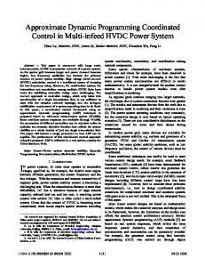
Fig. 14. Snapshot of 120 scans (2 minutes) when , , and and , respectively. Axes units are in km, the search area is (b) and (c) are the outputs for true targets’ trajectories.

Fig. 9 shows versus —i.e., the receiver operating characteristic (ROC)—for when and scans are integrated. is reported in logarithmic scale, and different values of are considered. Observe that, when , the curve for a given level ends when , since this is the largest admissible FAR. Moreover, these curves have a smaller slope than PD for the traditional scheme , which means that the proposed two-stage scheme is less sensitive to threshold’s variations: to give an example, in the range , while PD of the traditional scheme increase from 0.35 to 0.61, for is always around 0.6 for . It is also interesting to notice that, when varies, the ROC curves of the proposed two-stage scheme describe a region, which lies above the ROC curve of the traditional scheme: therefore, a better performance can be achieved and a larger freedom is given at the system design stage. In the second set of figures, is increased up to approximately Mach-2. Figs. 10 and 11 show PD and RMSE versus , respectively, for different values of SDR when and scans are integrated, and , while Figs. 12 and 13 consider the same scene when . A comparison with Figs. 5 and 6 shows that almost no loss is incurred when , so that large gains with respect to the traditional scheme are possible even in the detection of fast maneuvering targets. When is increased to values larger than , the detection gain remain almost unchanged, but the accuracy in the position estimation degrades, and, when

: (a) is the input of the second stage, while and 40 to 140 km, and the red curves denote the

, it becomes poorer than that of the traditional scheme. We remark, however, that these values of are not of interest, as the computational complexity needed to run Algorithm 1 may become unaffordable. In Fig. 14 we report a short data snapshot of 120 scans (i.e., 2 minutes) for , , and . The black dots represent the alarm’s positions, while the red straight lines indicate the true target trajectories. Plot (a) reports the input of the second stage, while Plots (b) and (c) refer to the outputs when and , respectively. It is seen that the proposed two-stage scheme is able to confirms 1030 alarms, as opposite to the 619 alarms of the traditional scheme, and all these alarms are correctly located along the true target trajectories. Finally, for comparison purposes, we analyze the case where the primary threshold , and the detection architecture in Fig. 2 reduces to the detectors operating on raw input data considered in [2]–[4], [25]. To limit the computational burden, we restrict the search area to and 98 to 102 km, where one target with velocity up to is simulated. The scan period is 1 s, , and all other parameters remains unchanged. Fig. 15 reports versus SDR for different values of when and scans are integrated, while Fig. 16 shows the corresponding RMSE’s on the estimated target position. Similarly to the previous plots, increases monotonically with , showing here a gap of about 10 dB at between the traditional scheme in Fig. 1

GROSSI et al.: TBD IN RADAR SYSTEMS

Fig. 15. Detection probability at the output of the second stage versus SDR for . The search area is and 98 to 102 km. different values of

Fig. 16. Root mean square error on the estimated target position at the output . The search area of the second stage versus SDR for different values of and 98 to 102 km. is

and MFD with raw data ( and ). Any point between these two extrema can be achieved with proper selection of in the proposed scheme in Fig. 2, and complexity is traded for performance. As to , it is decreasing with SDR, but no strict ordering can be observed among different

2617

Fig. 17. Root mean square error on the estimated target trajectory at the output . The search area of the second stage versus SDR for different values of and 98 to 102 km. is

Fig. 18. Root mean square error on the estimated target range-rate at the output . The search area of the second stage versus SDR for different values of and 98 to 102 km. is

values of . Furthermore, it can be noticed that in the small SDR regime the detection gain with respect to the traditional scheme in Fig. 1 comes at the price of worse accuracy in the position estimation. In Figs. 17 and 18, instead, we analyze the performance of the procedure in terms of track estimation and

2618

IEEE TRANSACTIONS ON SIGNAL PROCESSING, VOL. 61, NO. 10, MAY 15, 2013

range-rate estimation, respectively,7 and is reported versus SDR for different values of and for . Again, there is no strict ordering among the different levels of , but it can be observed that delivers, with negligible computational complexity increase with respect to the traditional scheme, a gain in the detection probability, a higher accuracy in the position estimation over a wide range of SDR’s (corresponding to ), and a range-rate information (otherwise not available).

where . The uncertainty so as to can be removed by maximizing over the set of admissible trajectories , and the generalized likelihood ratio test (see [49]) amounts to compare with a threshold the statistic

V. CONCLUSION In this work we have proposed and analyzed a two-stage architecture for target detection in radar systems, wherein a TBD processor operates on a set of candidate plots provided by the Detector and Plot-Extractor. A novel dynamic programming algorithm, which does not require a discretization of the state space, has been derived for plot validation. The complexity analysis reported in Section III-E has shown that in standard radar scenarios the proposed algorithm has a computational complexity which can be much lower than that of a multi-frame detection procedure based on the Viterbi algorithm (hardly amenable to a real-time implementation when the number of sensor resolution elements is large). Additionally, the numerical analysis in Section IV has shown that the proposed two-stage detection procedure guarantees a large detection gain with respect to the standard radar processing operating at the same level of false alarm rate. APPENDIX Assume that thresholding, and that sities of whenever spectively, and denote in (2) is8

, as a result of the first stage . Let and be the denis a false or a true alarm, re. Then the density of

whether it is a true alarm or not, respectively, where is the indicator function of the event . Let be the trajectory of the target, and assume scan-to-scan independence conditioned on the absence or presence of a target with this trajectory, then the log-likelihood ratio of is

7Track estimates are side results of the energy integration process, and they can be exploited to extract range-rate information. We remark here that they are not long continuous tracks in terms of Cartesian position and velocity, as it happens in standard tracking, but small tracklets in term of range-azimuth measurements only, which can be possibly used by the following tracking stage to form long continuous tracks. 8It is a mixed (discrete/continuous) random variables, and the density is computed with respect to the measure defined as the sum of the Dirac measure centered in and the Lebesgue measure.

(7)

where it has been exploited the fact that if Observe that if is an affine, increasing function, i.e., , , then (7) is equivalent to

.

which corresponds to (3) if is set equal to . E.g., if and are densities of exponential distributions with location parameter and scale parameter and , respectively, with (i.e., , which is a common model for radar measurements), then is affine and increasing. REFERENCES [1] S. Blackman and R. Popoli, Design and Analysis of Modern Tracking Systems. Norwood , MA, USA: Artech House, 1999. [2] S. W. Shaw and J. F. Arnold, “Design and implementation of a fully automated OTH radar tracking system,” in IEEE Proc. Int. Radar Conf., Alexandria, VA, USA, May 1995, pp. 294–298. [3] P. Wei, J. Zeidler, and W. Ku, “Analysis of multiframe target detection using pixel statistics,” IEEE Trans. Aerosp. Electron. Syst., vol. 31, no. 1, pp. 238–247, Jan. 1995. [4] H. Im and T. Kim, “Optimization of multiframe target detection schemes,” IEEE Trans. Aerosp. Electron. Syst., vol. 35, no. 1, pp. 176–186, Jan. 1999. [5] Y. Barniv, “Dynamic programming solution for detecting dim moving targets,” IEEE Trans. Aerosp. Electron. Syst., vol. 21, no. 1, pp. 144–156, Jan. 1985. [6] J. F. Arnold, S. W. Shaw, and H. Pasternack, “Efficient target tracking using dynamic programming,” IEEE Trans. Aerosp. Electron. Syst., vol. 29, no. 1, pp. 44–56, Jan. 1993. [7] S. M. Tonissen and R. J. Evans, “Performance of dynamic programming techniques for track-before-detect,” IEEE Trans. Aerosp. Electron. Syst., vol. 32, no. 4, pp. 1440–1451, Oct. 1996. [8] W. R. Blanding, P. K. Willett, Y. Bar-Shalom, and R. S. Lynch, “Directed subspace search ML-PDA with application to active sonar tracking,” IEEE Trans. Aerosp. Electron. Syst., vol. 44, no. 1, pp. 201–216, Jan. 2008. [9] N. C. Mohanty, “Computer tracking of moving point targets in space,” IEEE Trans. Pattern Anal. Mach. Intell., vol. 3, no. 5, pp. 606–611, Sep. 1981. [10] I. S. Reed, R. M. Gagliardi, and H. M. Shao, “Application of threedimensional filtering to moving target detection,” IEEE Trans. Aerosp. Electron. Syst., vol. 19, no. 9, pp. 898–905, Nov. 1983. [11] Y. Barniv and O. Kella, “Dynamic programming solution for detecting dim moving targets. Part II: Analysis,” IEEE Trans. Aerosp. Electron. Syst., vol. 23, no. 6, pp. 776–788, Nov. 1987. [12] I. Reed, R. Gagliardi, and L. Stotts, “Optical moving target detection with 3-D matched filtering,” IEEE Trans. Aerosp. Electron. Syst., vol. 24, no. 4, pp. 327–336, Jul. 1988. [13] I. Reed, R. Gagliardi, and L. Stotts, “A recursive moving-target-indication algorithm for optical image sequences,” IEEE Trans. Aerosp. Electron. Syst., vol. 26, no. 3, pp. 434–440, May 1990. [14] H. M. Shertukde and Y. Bar-Shalom, “Detection and estimation for multiple targets with two omnidirectional sensors in the presence of false measurements,” IEEE Trans. Acoust., Speech, Signal Process., vol. 38, no. 5, pp. 749–763, May 1990. [15] Y. T. Chan, G. H. Niezgoda, and S. P. Morton, “Passive sonar detection and localization by matched velocity filtering,” IEEE J. Ocean. Eng., vol. 20, no. 3, pp. 179–189, Jul. 1995.

GROSSI et al.: TBD IN RADAR SYSTEMS

[16] T. Kirubarajan and Y. Bar-Shalom, “Low observable target motion analysis using amplitude information,” IEEE Trans. Aerosp. Electron. Syst., vol. 32, no. 10, pp. 1367–1384, Oct. 1996. [17] S. M. Tonissen and Y. Bar-Shalom, “Maximum likelihood track-before-detect with fluctuating target amplitude,” IEEE Trans. Aerosp. Electron. Syst., vol. 34, no. 3, pp. 796–806, Jul. 1998. [18] J. D. R. J. Kramer and W. S. Reid, “Track-before-detect processing for an airborne type radar,” in Proc. IEEE Int. Radar Conf., Arlington, VA, May 1990, pp. 422–427. [19] J. L. Harmon, “Track-before-detect performance for a high prf search mode,” in Rec. IEEE Nat. Radar Conf., Los Angeles, CA, Mar. 1991, pp. 11–15. [20] B. D. Carlson, E. D. Evans, and S. L. Wilson, “Search radar detection and track with the Hough transform. Part I: System concept,” IEEE Trans. Aerosp. Electron. Syst., vol. 30, no. 1, pp. 102–108, Jan. 1994. [21] B. D. Carlson, E. D. Evans, and S. L. Wilson, “Search radar detection and track with the Hough transform. Part II: Detection statistics,” IEEE Trans. Aerosp. Electron. Syst., vol. 30, no. 1, pp. 109–115, Jan. 1994. [22] B. D. Carlson, E. D. Evans, and S. L. Wilson, “Search radar detection and track with the Hough transform. Part II: Detection performance with binary integration,” IEEE Trans. Aerosp. Electron. Syst., vol. 30, no. 1, pp. 116–125, Jan. 1994. [23] W. R. Wallace, “The use of track-before-detect in pulse-Doppler radar,” in Proc. IEEE Int. Radar Conf., Edinburgh, U.K., Oct. 2002, pp. 315–319. [24] S. Buzzi, M. Lops, and L. Venturino, “Track-before-detect procedures for early detection of moving target from airborne radars,” in Proc. IEEE Int. Radar Conf., Toulouse, France, Oct. 2004. [25] S. Buzzi, M. Lops, and L. Venturino, “Track-before-detect procedures for early detection of moving target from airborne radars,” IEEE Trans. Aerosp. Electron. Syst., vol. 41, no. 3, pp. 937–954, Jul. 2005. [26] D. Orlando, L. Venturino, M. Lops, and G. Ricci, “Space-time adaptive algorithms for track-before-detect in clutter environments,” in Proc. IEEE Int. Radar Conf., Bordeaux, France, Oct. 2009. [27] M. Lops, M. Mancino, D. Orlando, G. Ricci, and L. Venturino, “A model-based track-before-detect strategy,” in Proc. Eur. Radar Conf., Paris, France, Oct. 2010. [28] D. Orlando, L. Venturino, M. Lops, and G. Ricci, “Track-before-detect strategies for STAP radars,” IEEE Trans. Signal Process., vol. 58, no. 2, pp. 933–938, Feb. 2010. [29] D. Orlando, G. Ricci, and Y. Bar-Shalom, “Track-before-detect algorithms for targets with kinematic constraints,” IEEE Trans. Aerosp. Electron. Syst., vol. 47, no. 3, pp. 1837–1849, Jul. 2011. [30] S. D. Blostein and T. S. Huang, “Detecting small, moving objects in image sequences using sequential hypothesis testing,” IEEE Trans. Signal Process., vol. 39, no. 7, pp. 1611–1629, Jul. 1991. [31] R. Perry, A. Vaddiraju, and K. Buckley, “Multitarget list Viterbi tracking algorithm,” in Proc. Asilomar Conf. Signals, Syst. Comput., Pacific Grove, CA, Nov. 1998, pp. 436–440. [32] S. Buzzi, M. Lops, and L. Venturino, “Track-before-detect procedures in multi-targets environments,” in Proc. IEEE Int. Waveform Diversity and Design Conf., Lihue, HI, USA, Jan. 2006, pp. 422–427. [33] S. Buzzi, M. Lops, L. Venturino, and M. Ferri, “Detection of an unknown number of targets via track-before-detect procedures,” in Proc. IEEE Radar Conf., Boston, MA, USA, Apr. 2007, pp. 180–185. [34] W. R. Blanding, P. K. Willett, Y. Bar-Shalom, and R. S. Lynch, “Multiple target tracking using maximum likelihood probabilistic data association,” in Proc. IEEE Aerosp. Conf., Big Sky, MT, Mar. 2007. [35] S. Buzzi, M. Lops, L. Venturino, and M. Ferri, “Track-before-detect procedures in a multi-target environment,” IEEE Trans. Aerosp. Electron. Syst., vol. 44, no. 3, pp. 1135–1150, Jul. 2008. [36] E. Grossi and M. Lops, “Multi-frame sequential procedures in early warning surveillance radar systems,” in IEEE Radar Conf., Rome, Italy, May 2008, pp. 1–6. [37] E. Grossi and M. Lops, “Joint sequential detection and estimation of Markov targets,” in Proc. IEEE Inf. Theory Workshop, Porto, Portugal, May 2008, pp. 308–312. [38] E. Grossi and M. Lops, “Sequential along-track integration for early detection of moving targets,” IEEE Trans. Signal Process., vol. 56, no. 8, pp. 3969–3982, Aug. 2008. [39] E. Grossi and M. Lops, “Sequential detection of markov targets with trajectory estimation,” IEEE Trans. Inf. Theory, vol. 54, no. 9, pp. 4144–4154, Sep. 2008. [40] G. D. J. Forney, “The Viterbi algorithm,” Proc. IEEE, vol. 29, no. 3, pp. 268–277, Mar. 1973. [41] P. Uruski and M. Sankowski, “On estimation of performance of trackbefore-detect algorithm for 3D stacked-beam radar,” in Proc. Int. Conf. Microwaves, Radar, Wireless Commun. (MIKON), Warsaw, Poland, May 2004, pp. 97–100.

2619

[42] E. Grossi, M. Lops, and L. Venturino, “Track-before-detect with censored observations,” in Proc. IEEE Int. Conf. Acoust., Speech, Signal Process. (ICASSP), Kyoto, Japan, Mar. 2012, pp. 3941–3944. [43] E. Grossi, M. Lops, and L. Venturino, “A two-step multi-frame detection procedure for radar systems,” in Proc. Int. Conf. Inform. Fusion (FUSION), Singapore, Jul. 2012, pp. 1196–1201. [44] E. Grossi, M. Lops, and L. Venturino, “A track-before-detect procedure for sparse data,” in Proc. IEEE Statist. Signal Process. Workshop (SSP), Ann Arbor, MI, USA, Aug. 2012, pp. 772–775. [45] E. Grossi, M. Lops, and L. Venturino, “Detection validation in radar systems via along-track integration,” in Proc. IET Int. Radar Conf. (RADAR), Glasgow, Scotland, Oct. 2012. [46] J. B. Taylor, An Introduction to Error Analysis: The Study of Uncertainties in Physical Measurements, 2nd ed. New York, NY, USA: Univ. Sci. Books, 1997. [47] L. R. Rabiner, “A tutorial on hidden markov models and selected applications in speech recognition,” Proc. IEEE, vol. 77, no. 2, pp. 257–286, Feb. 1989. [48] X. Rong Li and V. P. Jilkov, “Survey of maneuvering target tracking. Part I: Dynamic models,” IEEE Trans. Aerosp. Electron. Syst., vol. 39, no. 4, pp. 1333–1364, Oct. 2003. [49] H. L. V. Trees, Detection, Estimation, and Modulation Theory—Part I. New York, NY, USA: Wiley, 2001.

Emanuele Grossi (M’08) was born in Sora, Italy, on May 10, 1978. He received the Dr. Eng. degree (with honors) in telecommunication engineering in 2002 and the Ph.D. degree in electrical engineering in 2006, both from the University of Cassino, Italy. In 2005, he was a Visiting Scholar with the Department of Electrical and Computer Engineering, University of British Columbia, Canada, and in 2009 he had a visiting appointment with the Digital Technology Center, University of Minnesota, Minneapolis. Since February 2006, he has been an Assistant Professor at the University of Cassino, Italy. His research interests concern wireless communication systems, radar detection and tracking, and statistical decision problems with emphasis on sequential analysis.

Marco Lops (M’96–SM’01) was born in Naples, Italy, on March, 16 1961. He received the “Laurea” and Ph. D. degrees from “Federico II” University, Naples. From 1989 to 1991, he was an Assistant Professor and from 1991 to 2000, an Associate Professor, with “Federico II” University. Since March 2000, he has been a Professor at the University of Cassino, Italy, and, during 2009–2011, he was also with ENSEEIHT, Toulouse, France. In fall 2008, he was a Visiting Professor with the University of Minnesota, Minneapolis, and in spring 2009, with Columbia University, New York. His research interests are in detection and estimation, with emphasis on communications and radar signal processing.

Luca Venturino (S’03–M’06) received the Dr. Eng. degree (with honors) in telecommunication engineering in 2002, and the Ph.D. degree in electrical engineering in 2006, both from the Università degli Studi di Cassino, Italy. He is now an Assistant Professor with the Department of Electrical and Information Engineering, Università degli Studi di Cassino e Lazio Meridionale, Italy, engaged in research and teaching activities on telecommunications. His research interests concern resource allocation in cellular networks, space-time signal processing in wireless multiple-input multiple-output systems, and signal detection in radar. In 2004 and 2009, he was a Visiting Scholar with the Department of Electrical Engineering, Columbia University, New York. Between 2006 and 2008, he spent eight months at NEC Laboratories America, Princeton, NJ, as Research Associate.