Proceedings of the 3rd International Conference on Systems and Control, Algiers, Algeria, October 29-31, 2013
WeBC.1
A Quadratic Programming Optimization for Dynamic Economic Load Dispatch: comparison with GAMS F. Benhamida, I. Ziane(1), S. Souag
Y. Salhi, B. Dehiba(2)
Irecom laboratory, dept. of electrotechnics UDL university of Sidi Bel Abbes Sidi Bel Abbes, Algeria (1)
[email protected]
Apelec laboratory, dept. of electrotechnics UDL university of Sidi Bel Abbes Sidi Bel Abbes, Algeria (2)
[email protected]
Abstract— This paper presents a comparative analysis study of an efficient and reliable quadratic programming (QP) and general algebraic modeling system (GAMS) to solve dynamic economic load dispatch (DELD) problem with considering transmission losses in a power system. The proposed QP method takes care of different unit and system constraints to find optimal solution. To validate the effectiveness of the proposed QP and GAMS solution, simulations have been performed using two different cases, a 18-unit, 40-unit. Results obtained with the QP method and GAMS-CONOPT solver have been compared with other existing relevant approaches available in literatures. Experimental results show a proficiency of the QP method over other existing techniques in terms of robustness and its optimal search behavior comparing to GAMS.
load dispatch; quadratic Keywords – Economic programming; general algebraic modeling system GAMS; Ramp rate limit. I.
INTRODUCTION
Economic load dispatch (ELD) problem concern the determination of the optimal combination of power output for all generating units which will minimize the total fuel cost while satisfying load and operational constraints in a high voltage power system. ELD is a complex problem to solve because of its massive dimension, a non-linear objective function and large number of constraints. Various investigations on the ELD have been undertaken till date. Suitable improvements in the unit output scheduling can contribute to significant cost savings. To improve the quality of solution, lots of researches have been done and various methods have been evolved so far in the field of ELD [1], [2]. Classical optimization techniques, such as the lambda iteration approach, the gradient method, the linear programming method and Newton’s method were used to solve the ELD problem [3]. Lambda iteration method is the most common, which has been applied to solve ELD problems. But for effective implementation of this method, the formulation must be continuous. Though fast and reliable, the main drawback of the linear programming methods is that they are associated with the piecewise linear cost approximation [4]. Artificial Neural Network (ANN) techniques such as Hopfield Neural Network (HNN) [4] have been used to solve
ELD for units having continuous or piecewise quadratic fuel cost functions and for units having prohibited zone constraints. Hopfield energy function and numerical iterations are applied to minimize the energy function which is mapped to the objective function of the ELD problem. In the conventional Hopfield Neural Network, the input-output relationship for its neurons is described by sigmoid function. Due to the use of the sigmoid function, the Hopfield model suffers from large computational time and curve saturation. To avoid such problem problems, a linear model is also used [5]. Evolutionary programming (EP), genetic algorithm (GA), differential evolution (DE), particle swarm optimization (PSO) [6], [7] have been also proved to be effective with promising performance etc. Improved fast evolutionary programming algorithm has been successfully applied for solving the ELD problem [1], [5]. Chaotic particle swarm optimization (CPSO) [8], new particle swarm with local random search (NPSO-LRS) [9], Self-Organizing Hierarchical PSO [10], Bacterial foraging optimization [11], improved coordination aggregated based PSO [12], quantum-inspired PSO [13], improved PSO [14], HHS algorithm [15] and HIGA [16] have been successfully applied to solve the ELD problem. A comparative analysis study of Quadratic programming (QP) and General Algebraic Modeling System (GAMS) approach is proposed to solve ELD problems. QP is an effective tool to find global minima for optimization problem having quadratic objective function with linear constraints. The objective function for the 2 test system used in the simulation is quadratic but the constraints are not linear. Constraints are liberalized by transformation of variable technique and the QP is applied recursively till the convergence is achieved. GAMS is a high-level model development environment that supports the analysis and solution of mixed integer optimization linear, and non linear problems. GAMS is an accurate tool which can be useful easily for large and complex optimization problem. In this paper the effectiveness of the proposed algorithm is demonstrated using 2 test system (i) a 18-unit, (ii) a 40-unit. II.
ELD PROBLEM FORMULATION
In a power system, the unit commitment problem has various sub-problems varying from linear programming problems to complex non-linear problems. The concerned ELD problem is one of the different non-linear programming
978-1-4799-0275-0/13/$31.00 ©2013 IEEE
Proceedings of the 3rd International Conference on
WeBC.1
sub-problems of unit commitment, where the units are considered all on line for a specified tine interval. The ELD problem is about minimizing the fuel cost of generating units for a specific period of operation so as to accomplish optimal generation dispatch among operating units and in return satisfying the system load demand considering power system operational constraints. The objective function corresponding to the production cost can be approximated to be a quadratic function of the active power outputs from the generating units. Symbolically, it is represented as
(6)
PGimin ≤ PGi ≤ PGimax
3) Ramp Rate Limits: The range of actual operation of online generating unit is restricted by its ramp rate limits. These limits can impact the operation of generating unit. The operational decision at the present hour may affect the operational decision at the later hour due to ramp rate limits. Pi(t)
Pi(t)
Pi(t)+URi(t)
Pi(t+1)
Pi(t)-URi(t)
Pi(t) N
min FT ( PG ) = ∑ Fi ( PGi )
t
(1)
t+1
t
t
t+1
t+1
i =1
a) Steady state power demand
where the expression for cost function corresponding to i-th generating unit is given by: 2 i Gi
Fi ( PGi ) = a P + bi PGi + ci
(2)
Figure 1.
The objective function is subject to the following constraints:
Ramp rate limits of the generating units
The generator constraints due to ramp rate limits of generating units are given as
Pit − Pi ( t −1) ≤ URi B)
The total system generation must be equal to the sum total system loads (PD) and losses (PL). That is, (3)
(7)
when generation decreases Pi (t −1) + Pit ≤ DRi
1) Power Balance Constraints:
N
c) Decreased power demand
A) when generation increases
where ai , bi and ci are the cost coefficients; PGi is the real power output (MW) of i-th generator corresponding to time period t and N is the number of online generating units to be dispatched.
PD + PL = ∑ PGi
b) Increased power demand
(8)
Therefore the generator constraints can be modified as max( Pi min , Pi (t −1) − DRi ) ≤ Pit ≤ min( Pi max , Pi ( t −1) + URi )
(9)
i =1
The transmission losses can be expressed using the Bcoefficients loss formula N
N
N
i
j
i
PL ({ PGi } ) = ∑∑ PGi Bi , j Pn 2 + ∑ Bi ,0 .PGi + B0,0
(4)
where the parameters {Bi,,j}, {Bi,0}, and B0,0 are Bcoefficients known for a specific power system. By applying Lagrangian multipliers method and KuhnTucker conditions for unbounded inequality constraints, the following conditions for optimality can be obtained. N ⎛ ⎞ 2ai PGi + bi = λ ⎜ 1 − Bi ,0 − 2∑ Bi , j PGi ⎟ (i = 1, 2,..., N ) j =1 ⎝ ⎠
(5)
III.
ECONOMIC DISPATCH PROBLEM SOLUTION BY COMPACT QUADRATIC PROGRAMMING
QP is an effective optimization method to find the global solution if the objective function is quadratic and the constraints are linear. It can be applied to optimization problems having non-quadratic objective and nonlinear constraints by approximating the objective to quadratic function and the constraints as linear. QP is the mathematical problem of finding a vector x that minimizes a quadratic function (23): 1 min ( x T H x + f ' x) , x 2
(10)
Subject to the linear inequality (8), equality (9) and bound constraints (10):
2) The Generator Constraints: The power generated by each generator should be within its lower limit and upper limit so that
978-1-4799-0275-0/13/$31.00 ©2013 IEEE
Ax ≤ b
(11)
Aeq x = beq
(12)
lb ≤ x ≤ ub
(13)
Proceedings of the 3rd International Conference on
WeBC.1
To map the ED to QP, the objective function variables are given by the power generation output vector as follow: (14)
x = [ PG 1 , PG 2 ,..., PGN ]T
a1 ⎡ ⎤ 0 ⎢1 − 2 B P − B " ⎥ 11 G1 01 ⎢ ⎥ # % # ⎥ H = 2× ⎢ ⎢ ⎥ aN ⎢ ⎥ " 0 ⎢⎣ 1 − 2BNN PGN − B0 N ⎥⎦
⎡ ⎤ bN b1 f =⎢ ,..., ⎥ − B P − B − B P − B 1 2 1 2 NN GN 11 G 1 01 0N ⎦ ⎣
T
(15)
T
(16)
IV.
GENERAL ALGEBRAIC MODELING SYSTEM (GAMS)
GAMS is a high-level model specially designed for modeling linear, nonlinear and mixed integer optimization problems. GAMS can easily handle large and complex problems. It is especially useful for handling large complex problems, which may require much revision to establish an accurate model. Models can be developed, solved and documented simultaneously, maintaining the same GAMS model file. Apart from a wide variety of optimization problems, it can handle simultaneous linear and non-linear equation systems and further development would include (linear and non-linear) complementarity problems and general equilibrium problems. The basic structure of a mathematical model coded in GAMS has the components: sets, data, variable, equation, model and output [18] and the solution procedures are shown below. Optimization Model Formulation in GAMS
To satisfy the equality constraint Aeq* x = beq, we set Model description, preprocessing, solver
(17)
beq = PD + (1 + z ) PL
Where PD is a power demand and PL is losses calculated by (4) and z is a controlling parameters. ⎛ ⎡ B11 ... B1N ⎜ Aeq = [1, 1,...,1] + z. ⎜ [ P1 , P2 ,..., PN ] ⎢⎢ # % # ⎜ ⎢⎣ BN1 " BNN ⎝
[ B01," B0 N ] + [
⎤ ⎥+ ⎥ ⎥⎦
Global and Local search method for nonlinear optimization
Optional calls for other solvers and external Programs
(18)
Figure 2. GAMS modeling and solution procedure.
B00 B00 B ⎞ , ,..., 00 ] ⎟ P1 P2 PN ⎠
The limits of power generated are imposed in the formulation of QP as follows: min min lb = [ PGmin 1 , PG 2 ,..., PGN ]
(19)
max max ub = [ PGmax 1 , PG 2 ,..., PGN ]
(20)
Step 1: Initialize the procedure, allocate lower limit of each unit, and evaluate the transmission loss PL old. Step 2: Calculate H, f, beq, Aeq, lb, ub using (15)-(20) respectively. Step 3: Determine the power allocation of each plant by substitute the quantities of step 2 in the quadratic programming solver to determine the corresponding optimal power generations PGi , i = 1,..,N. Step 4: Calculate the new value of transmission losses PLnew using (7) by substituting the power generation determined in step 3. Step 5: Check for convergence N
GAMS solution report
PD + PLnew − ∑ PGi ≤ ε
(21)
GAMS formulation follows the basic format as given below: • Sets: Declaration, Assignment of members; •
Data (parameters, tables, scalars), Declaration, Assignment of values;
•
Variables: Declaration, Assignment of type, Assignment of bounds and/or initial values (optional);
•
Equations: Declaration, Definition;
•
Model and solve statements;
•
Display statements (optional)
V.
RESULT AND DISCUSSION
The QP and a GAMS-CONOPT solver have been applied on 2 different standard high voltage power systems. Test case I is a 18-unit, Test case II is a 40-unit.The programs were written in MATLAB 7.8 for QP and implementation on GAMS with a Pentium 4 processor and 1GB RAM.
i =1
where ε is the tolerance value, for power balance violation. Step 6: Carry out the steps 2-5 till convergence is achieved.
A. 18-Unit test sytem A 18-unit test system having quadratic cost function: The parameters of all thermal units are taken from [18], and given in Table I. The maximum power demand of the system set at PD = 433.22 MW. The results are compared with λ-iteration and Binary GA [18], RGA [18] and ABC [21] for this
978-1-4799-0275-0/13/$31.00 ©2013 IEEE
Proceedings of the 3rd International Conference on
WeBC.1
system. The summarized and comparative results of test case 1 for different demands (95%, 90%, 80% and 70%) without losses. From Table I, we can show that QP and CONOPTGAMS solver both provides superior result then earlier reported results; but GAMS provides much better result than QP. The summarized and comparative DELD results of case 1 are given Table II (between QP and GAMS). The percent changes in results are also given in Table II and illustrated in Fig. 2. TABLE I. Unit n° 1 2 3 4 5 6 7 8 9 10 11 12 13 14 15 16 17 18
Pimi
percent changes in results are also given in Table VI and illustrated in Fig. 3. TABLE II. Unit n° 1 2 3 4 5 6 7 8 9 10 11 12 13 14 15 16 17 18 19 20 21 22 23 24 25 26 27 28 29 30 31 32 33 34 35 36 37 38 39 40
PARAMETERS OF 18-UNIT SYSTEM
n
Pimax
ai
bi
ci
Rdown
Rup
7 7 13 16 16 3 3 3 3 3 3 3 3 3 3 3 3 3
15.00 45.00 25.00 25.00 25.00 14.75 14.75 12.28 12.28 12.28 12.28 24.00 16.20 36.20 45.00 37.00 45.00 16.20
0.602842 0.602842 0.214263 0.077837 0.077837 0.734763 0.734763 0.514474 0.514474 0.514474 0.514474 0.657079 1.236474 0.394571 0.420789 0.420789 0.420789 1.236474
22.45526 22.45526 22.52789 26.75263 26.75263 80.39345 80.39345 13.19474 13.19474 13.19474 13.19474 56.70947 84.67579 59.59026 56.70947 55.96500 55.96500 84.67579
85.74158 85.74158 108.98370 49.06263 49.06263 677.73000 677.73000 44.390000 44.390000 44.390000 44.390000 574.96030 820.37760 603.02370 567.93630 567.93630 567.93630 820.37760
10 10 10 10 10 5 10 10 10 10 10 10 10 7 10 10 10 3
10 10 10 10 10 5 10 10 10 10 10 10 10 7 10 10 10 3
B. 40-Unit test sytem A 40-unit with quadratic cost functions where the input data of the entire system are given in [22], and given in Table II. A load demands of 9000 MW and 10500 MW without transmission losses are considered. The results are compared with VSDE [22] and SA [21] methods for this system. The results obtained by QP approach and CONOPT algorithm under the optimization environment GAMS are listed in Table III. The 10 load demands are posed for study the DELD problem and the results are listed in Table VI. The TABLE III.
PARAMETERS OF 40-UNIT SYSTEM
Pimin
Pimax
ai
bi
40 60 80 24 26 68 110 135 135 130 94 94 125 125 125 125 125 220 220 242 242 254 254 254 254 254 254 10 10 10 20 20 20 20 18 18 20 25 25 25
80 120 190 42 42 140 300 300 300 300 375 375 500 500 500 500 500 500 500 550 550 550 550 550 550 550 550 150 150 150 70 70 70 70 60 60 60 60 60 60
0.03073 0.02028 0.00942 0.08482 0.09693 0.01142 0.00357 0.00492 0.00573 0.00605 0.00515 0.00569 0.00421 0.00752 0.00708 0.00708 0.00708 0.00313 0.00313 0.00313 0.00313 0.00298 0.00298 0.00284 0.00284 0.00277 0.00277 0.52124 0.52124 0.52124 0.25098 0.16766 0.26350 0.30575 0.18362 0.32563 0.33722 0.23915 0.23915 0.23915
8.3360 7.0706 8.1817 6.9467 6.5595 8.0543 8.0323 6.9990 6.6020 12.908 12.986 12.796 12.501 8.8412 9.1575 9.1575 9.1575 7.9691 7.9550 7.9691 7.9691 6.6313 6.6313 6.6611 6.6611 7.1032 7.1032 3.3353 3.3353 3.3353 13.052 21.887 10.244 8.3707 26.258 9.6956 7.1633 16.339 16.339 16.339
ci
Rdown
Rup
170.44 309.54 369.03 135.48 135.19 222.33 287.71 391.98 455.76 722.82 635.20 654.69 913.40 1760.4 1728.3 1728.3 1728.3 647.85 949.69 947.83 647.81 785.96 785.96 794.53 794.53 801.32 801.32 1055.1 1055.1 1055.1 1207.8 810.79 1247.7 1219.2 641.43 1112.8 1044.4 832.24 834.24 1035.2
20 40 50 10 10 40 80 80 80 80 80 80 80 80 80 80 80 80 80 80 80 80 80 80 80 80 80 80 80 80 20 20 20 20 15 20 20 20 20 20
20 40 50 10 10 40 100 100 100 100 130 130 100 100 100 100 100 100 100 100 100 100 100 100 100 100 100 100 100 100 40 40 40 20 20 40 40 40 40 40
COMPARISION OF ECONOMIC LOAD DISPATCH RESULT OF 18-UNIT
Demand
λ-iteration ($/hr)[19]
Binary GA ($/hr) [19]
Real coded GA ($/hr) [19]
ABC ($/hr) [20]
QP ($/hr)
411.559 389.898 346.576 303.254
29731.05 27652.47 23861.58 20393.43
29733.42 27681.05 23980.24 20444.68
29731.05 27655.53 23861.58 20396.39
29730.8 27653.3 23859.4 20391.6
29731.067 27653.750 23855.286 20386.216
TABLE IV.
COMPARAISON OF DELD RESULTS OF 18-UNIT SYSTEM WITH RAMP RATE LIMIT CONSTRAINTS USING QP AND GAMS GAMS
QP
Percent change (%)
Time interval
PD
Total cost
System λ
Total cost
System λ
Total cost
1 2 3 4
411.559 389.898 346.576 303.254
29731.067 27654.110 23856.274 20389.390
100.535 92.245 83.817 75.770
29731.066 27654.098 23856.301 20389.449
100.535 92.244 83.828 75.769
0,000003 0,000043 -0,000113 -0,000289
TABLE V. VSHDE [23]
Total generation PD (MW) Total cost ($/hr)
CONOPT solver ($/hr) 29731.067 27653.750 23855.286 20386.216
10500 10500 143943.9
System λ 0,0000 0,0011 -0,0131 0,0013
BEST POWER OUTPUT FOR 40-UNIT SYSTEM
SA [22]
QP
GAMS
10500 10500 143930.409
10500 10500 143926.424
10500 10500 143926.424
VCHDE [23]
9000 9000 121253.01
SA [22]
QP
9000 9000 121245.164
9000 9000 121244.086
978-1-4799-0275-0/13/$31.00 ©2013 IEEE
CONOPT 9000 9000 121244.086
Proceedings of the 3rd International Conference on TABLE VI.
WeBC.1
COMPARAISON OF DELD RESULTS OF 40-UNIT SYSTEM WITH AND RAMP RATE LIMIT CONSTRAINTS USING QP AND GAMS GAMS Time interval
PD
1 2 3 4 5 6 7 8 9 10
5000 5800 6200 7000 8400 9000 10500 9200 8700 8000
Total cost 79233.084 86515.540 90313.561 98152.380 113392.395 121244.086 143926.424 124066.733 117175.216 108761.503
System λ 8.813 9.384 9.597 10.040 12.119 13.943 16.257 14.282 13.100 11.196
QP
Percent change (%)
Total cost 79233.083 86515.539 90313.561 98152.379 113392.395 121244.086 143926.424 124066.733 117175.216 108761.503
System λ 8.812 9.383 9.596 10.040 12.118 13.943 16.257 14.282 13.100 11.195
Total cost 0.0000 0.0000 0.0000 0.0000 0.0000 0.0000 0.0000 0.0000 0.0000 0.0000
System λ 0.0113 0.0106 0.0104 0.0000 0.0082 0.0000 0.0000 0.0000 0.0000 0.00893
1,0
1,0
0,08
0,000
0,8
0,8
0,000
0,04 0,6
-0,001
0,6
-0,001
0,00 0,4 Total cost (%) System λ (%)
-0,002
0,4 -0,04
Total cost (%) System λ (%)
-0,002
0,2
0,2
-0,08 0,0
-0,003 1
2
Time interval (h)
3
0,0
-0,003
4
1
2
3
4
5
6
7
8
9
0,08 0,04 0,00 -0,04 -0,08
10
Time interval (h)
Figure 3. Percent variation in dynamic economic dispatch solution of the 18-generator problem for the 4 hour time interval using QP with ramping rate constraint comparing to CONOPT solver optimal solution without ramping rate constraints.
VI.
CONCLUSION
A QP approach and CONOPT-GAMS for optimization have been used for solving 2 test of high voltage power systems. Case I is 18-unit with quadratic cost characteristics without transmission loss, which is investigated by change in percentage of maximum demand (95%, 90%, 80% and 70%) and comparison is made with λiteration, Binary GA, RGA and ABC. Based on the simulated results, the QP and GAMS provides superior result than previously reported methods. Case III (40-unit) is investigated through two load demand levels and comparison is made with VSDE and SA. SGA and Hybrid GA reported in literature, the result shows that QP and GAMS performs better then above mentioned methods. The QP and CONOPT algorithm has superior features, including quality of solution and good computational efficiency, but GAMS provides much better result than QP. The results show that CONOPT algorithm is a promising technique for solving complicated problems in power system.
[2]
[3] [4]
[5]
[6]
[7]
[8]
[9]
REFERENCES [1]
Figure 4. Percent variation in dynamic economic dispatch solution of the 40-generator problem for the 10 hour time interval using QP with ramping rate constraint comparing to CONOPT solver optimal solution without ramping rate constraints.
B. H. Choudhary and S. Rahman, A review of recent advances in economic dispatch, IEEE Trans Power Sys., Vol. 5, No. 4, pp. 1248-1259, 1990.
[10]
H. H. Happ, Optimal power dispatches – a comprehensive survey, IEEE Trans. Power Apparatus Syst., PAS-96, pp. 841-854, 1971. A. J. Wood and B. F. Wollenberg, Power Generation, Operation and Control, Wiley., New York 2nd ed, 1996. J. H. Park, Y. S. Kim, I. K. Eom and K. Y. Lee, Economic Load Dispatch for pricewise Quadratic Cost Function Using Hopfield Neural, IEEE Trans. on Power Systems, Vol. 8, No. 3, pp. 1030-1038, 1993. F. Benhamida et al, “Generation allocation problem using a Hopfield bisection approach including transmission losses,” Elect. Power and Energ. Syst., vol. 33, no. 5, pp. 1165-1171, 2011. L. S. Coelho and V. C. Mariani, Combining of chaotic differential evolution and quadratic programming for economic dispatch optimization with valve-point effect, IEEE Trans. Power Syst., Vol. 21, No.2, pp. 989-996, 2006. J. B. Park, K. S. Lee, J. R. Shin and K.Y. Lee, A particle swarm optimization for economic dispatch with nonsmooth cost functions, IEEE Trans. Power Syst., Vol. 20, No. 1, pp. 34-42, 2005. A. Bhattacharya and P. K. Chattopadhyay, BiogeographyBased optimization for different economic load dispatch problems, IEEE Trans. Power Syst., Vol. 25, No. 2, pp. 10641077, 2010. C. Jiejin, M. Xiaoqian, L. Lixiang, and P. Haipeng, Chaotic particle swarm optimization for economic dispatch considering the generator constraints, Energy Converse Manage, Vol. 48, pp. 645-653, 2007. A. I. Selvakumar, and K. Thanushkodi, A new particle swarm optimization solution to non-convex economic dispatch
978-1-4799-0275-0/13/$31.00 ©2013 IEEE
Proceedings of the 3rd International Conference on
[11]
[12]
[13]
[14]
[15]
[16]
problem, IEEE Trans Power Syst., Vol. 22, No. 1, pp. 42-51, 2007. K. T. Chaturvedi, M. Pandit and L. Srivastava, SelfOrganizing Hierarchical Particle Swarm Optimization for Non-Convex Economic Dispatch, IEEE Trans. Power Syst., Vol. 23, No. 3, pp. 1079-1087,2008. B. K. Panigrahi and V. R. Pandi, Bacterial foraging optimization nelder mead hybrid algorithm for economic load dispatch, IET Gener. Transm. Distrib., Vol. 2, No. 4, pp. 556565, 2008. G. John Vlachogiannis and K. Y. Lee, Economic load dispatch – a comparative study on heuristic optimization techniques with an improved coordinated aggregation-based PSO, IEEE Trans. Power Syst., Vol. 24 , No. 2, pp. 991-1001, 2009. Ke Meng, H. G. Wang and Z. Y. Dong, Quantum-inspired particle swarm optimization for valve-point economic load dispatch, IEEE Trans. Power Syst., Vol. 25, No. 1, pp. 215222, 2010. J. B. Park, Y. W. Jeong, J. R. Sin and K. Y. Lee, An Improved particle swarm optimization for Non-convex Economic Load Dispatch Problems, IEEE Trans. Power Syst., Vol. 25, No. 1, pp. 156-166, 2010. V. R. Pandi, B. K. Panigrahi, R. C. Bansal, S. Das and A. Mohapatra, Economic load dispatch using hybrid swarm
WeBC.1
[17]
[18] [19]
[20]
[21]
[22]
intelligence based harmonics search algorithm, Electric Power Comp. and Systems, Vol. 39 pp. 751-767, 2011. M. M. Hosseini, H. Ghorbani, A. Rabii and Sh. Anvari, A novel heuristic algorithm for solving Non-convex economic load dispatch problem with non smooth cast function, J. Basic Appl. Sci. Res., 2(2)1130-1135, 2012. Sichard E. Rosenthal, GAMS, A User’s Guide, Tutorial GAMS Development Corporation, Washington, 2010. G. Ioannis, Damousis, G. Anastasios, G. Bakirtzis and S. Dokopoulos Petros, Network-Constrained Economic Dispatch Using Real-Coded Genetic Algorithm, IEEE Trans on power system, Vol. 18, No. 1, pp. 198-204, 2003. G. P. Dixit, H. M. Dubey, M. Pandit and B. K. Panigrahi, Economic Load Dispatch using Artificial Bee Colony Optimization, International Journal of Advances in Electronics Engineering, pp. 129-124, 2011. M. S. Kaurav, H. M. Dubey, M. Pandit and B. K. Panigrahi, Simulated Annealing Algorithm for Combined Economic and Emission Dispatch, International Conference, ICACCN pp. 631-636, 07-09 Oct 2011 Ji-Pyng Chiou, Variable Scaling hybrid differential evolution for large scale economic dispatch problem, Electrical power systems Reserch, Vol. 77, pp. 212-218, 2007.
978-1-4799-0275-0/13/$31.00 ©2013 IEEE