The rate of convergence of BP networks or TDNN is very low for multiclass problems, because some components of BP networks in multiclass classification hold ...
A Novel Fast Learning Algorithms for Time-Delay Neural Networks * Jiang Minghu Zhu Xiaoyan IEEE Member . . 0w-dcs@The State Key Lab of Intelligent Tech. & Systems, Dept. of Computer, Tsinghua University Beijing 100084, P.R.China Abstract: To counter the drawbacks that Waibel 's time-delay neural networks (TDW)take up long training time in phoneme recognition, the paper puts forward several improved fast learning methods of 1PW. Merging unsupervised Oja's rule and the similar error back propagation algorithm for initial training of 1PhW weights can effectively increase convergence speed, at the same time error firnction almost monotonyly descending. Improving error energy function. updating the changing of weights according to sue of output error, can increase training speed. From back propagation along layer, to average overlap part of back propagation error of first hidden layer along fiame, the training samples fiom a little to many gradually, convergence speed increases must faster. To multi-class phonemic modular 1PWs, we improve the architecture of Waible's modular networks, and get an optimum modular lDhWs (OMWs) of tree structure to accelerate its learning, Its training time is less than Waibel's modular TDWs. The convergence speed increases about tens of times when the complexity of network increases just a little more, and the recognized rate is the same on the whole. Keywora3: Phoneme Recognition, Time-delay neural networks, Convergencespeed, Optimum Module;
I. Introduction The Time-Delay Neural Network 0") [1,2] introduced by Waibel et al has achieved high performance for the data in isolated word utterances and the ability to tolerate the time lag caused by variations in the phoneme extraction position (time-shifting invariance). That is, the time-delay architecture is capable of capturing the dynamic nature of speech to achieve superior phoneme recognition performance. However, it has been found that this type neural network has the serious drawback that consumed a large amount of training time. The rate of convergence of BP networks or TDNN is very low for multiclass problems, because some components of BP
networks in multiclass classification hold back the change of output error in the initial iterations, and cause the increase of training time [3]. In order to solve this problem, A.Waibe1 [2] put forward to a module TDNN for classification of 23 Japanese phonemes, and picked up training speed of TDNN,Waibel's every modular network still exists multiclass problems and needs long training time. Anand [4] adopted a modular networks which transformed a k-class problem to a set of k two-class B D G o u t p u t layer h i d d e n layer 2 3 nodes h i d d e n layer 1 8 nodes
input layer 16 M e l
spectral coefficients ime, IS frames
F i g l . The structure o f T D N N
problems, and speedups the convergence rate of the networks; but Anand modular networks need train total sample data again for expanding new sample classes and take too many modular networks. Our aim is to find a O M " which the training time and number of module networks are less than ones of Anand module networks, easily expand new classes, and training time is also less than Waibel module networks. The part I1 is the structure of TDNN and fast learning algorithm. The part I11 is comparative experiment and the part IV is conclusion.
II. The Fast Algorithm of TDNN
.
The ChineseNational Natural Science Foundation and Chinese National PostdoctoralScience Foundation support the w r k
0-7803-5529-6/99/$10.00 01999 IEEE
1380
2.1 The Structure of TDNN Waibel's TDNN is shown in Fig1[13, the training take up a long training time, the calculating the energy errors of every layer has difference algorithms, they have a large effect to the convergence time of total TDNN. Suppose the weights of input layer to hidden layerl, hidden layer 1 to hidden 2, and hidden layer2 to out layer are 5!',)6,V$2),V$l separately, and L training samples {Xk},R = 1,2,-.,L. The expected output of k-th sample is yt = Q l t , y u , y 3 k }Output . of hidden layer 1 is: h::t = U(@\) = O(~C:.l~.:flV;~)X(m+,-I)I.t + V;!').-*(1)
Here rn = 1,2,..-,13 is h e in time sequence, i = 1,2,...,8., V,:) is threshold. Output of hidden layer 2 is: hZ!k = o(a::) =
2 3 Fast Learning Algorithm of TDNN: During the initial stage of training, the estimation error E is relatively large, the reduction of the total error is significant; however, when the estimation error decreases with training, the convergence of the algorithm becomes very slow. By modification of error backpropagation equation in order to accelerate its convergence. The energy function is defined by G(A)= AE+(l-A)E,, During the initial stage of training A=1, E is dominant and convergence speed is fast. When the error decreases with training, A from 1+0, but E, convergence is very fast when A +0. If activation function is tanho and error energy function is [6]:
c(a)=f i +(1 -a)E,
~(x~=l~~=lV;~~~~~~,-l)l.k + V;f').+) = o ~ ~ ~ ~ , -iJ' ~ ~ , C y , t +
Here rn = 12,. ,9 is frame in time sequence, i = 123 . V , f ) is threshold. Output of output layer is: 1.
-
~
~
~
~
,
~
~
,
~
~
gradient descent algorithm:
- W,,k-, = -VdG(A) law, = -V(JG(A) 1de,., )(de,.* 1aw,1 W,.k
= 661.t= ) 6 ~ ~ ~ l % , h ~ ~ - l )+%0)"'(3) . k Here i = 1,2,3; Tois threshold.
E=
~
= 0 5 ~ ~ ~ = , Z : =+(1-a).);r=t,x~=,yI.kel.t ,e,fk (10) Here A = exp(-p / E'). The weight adjustment adopt
9l.t
The error energy function is:
~
By error backpropagation, and from
~~=,x~J.h -h)' 12 = x:-,x:.le:t 12-44)
a(x) = tanh(x),d(x) = I-o'(x)
,we get:
w,,~ = w,,+, +q&;;(a)h:")...(ii) .
Here &:;(A) = ('-9;.t)cY,.k -4+,,,>*.*(12) The subscript of W is extended in (1 1) along time The unsupervised Oja's rule [6,7]initializes weight matrix of bottom layer. First initialize the bottom layer coordinate axle and get: W,, = W,&-,+ qa$ (A)hjti-,,M, weight matrix. Here p = 1,2,3;j = 1,2,.--,9;h~~~-,,),k = l,W,,,, is + (5) Calculate: i2!k= ~~,,C~~,,~f4),~~~~,-,,,.~ threshold. Update weighs V according to Oja's rule (Eq(6)): The weight adjustment from hidden layer 1 to layer 2 is:
2.2 Weight initialization:
Here a , /3 is a positive parameter separately. calculate: \.:' And
xm(fl),t
= x : . , c e , V ; ~ ~ ~ h t X ( ~ + j - l ) l . t (7)
= x:-~~(&t!,)t)vG!l) (8)
E? = ~:=~x~-~x~-~('~.k
- x C : . I ~ : ~ i V ; ~ ~ ~ h t ~ m C I J h t ) (''1
Repeat (5) to (9), until a convergence criterion is reached. M e r the unsupervised initializes weight matrix of bottom layer, the bottom layer weight matrix is kept fixed. A similar error back propagation algorithm initializes weight matrix of other layers. First, the output layer and the second hidden layer weights initialize small random values. Then, the weights of output layer are made convergence and then the weights of output layer and second hidden layer are made convergence by using similar error propagation of collect the sample in every sampleclasses. These adjustments are repeated until a convergence criterion is reached, after which the back propagation training begins.
1381
-
~
l
.
~
l
.
k
~
time coordinate axis, and given: (1) Vl(.C)J
= Vl::L)J-l
+
vx:l
&;:k
(w(pw-l)&,
(backpropagation along layer )
x:.,
And V112c,t = Vl::L-l +q Z 1 &::+r-l)l.k ( w ( m + r + . - z y , i (backpropagation from top to bottom along frame) here: &::+,-I)l.m
= [I-
initializes of weight matrix of bottom layer, a similar error back propagation algorithm initializes weight matrix of other layers. After initial training weights, get into the training of TDNN.Every method is as follow: Method 1: Without weight initialization. 0 5 A < 1,p = 1 , G(A) is as gradient error back-propagation, a(x)=trplh(x),
( ~ ~ ~ ~ , - l , , ) 2 1 C : . I ~ ~ n l *x ~ h l & ~ ! t ( ~ ) ~ ~ ~ X t
When V,):
is adjusted, X, = 1; rn = 1,2,...,9;p = 1,2,-.,13 (p, m are all time sequence), a = 1,2,3;c = 1,2,***,16;1= 12,. .-,8;r= 1,2,-..,5; The proposed method make the energy function updates weights according to size of output errors, and accelerate convergence speech when the estimation error decrease with training. The weights update criterion of error back propagation was changed from the average weights of all corresponding time-delay frames to the average drift overlap frames in first hidden layer. The samples training first makes a few number of sample convergence, then increase samples little by little and make them convergence.
2.4 The optimummodular neural networks: More the classes of BP networks are, more the weight change of output error is hold-back and more training time is need. Waibel's modular networks still exists multi-class classification and need long training time. A tree structure optimum modular neural networks ( O m s ) structure is proposed to fialfill the classification of multi-class problems. Each module network consists of a few submodule networks of tree structure, while each sub-module network only classifies two classes. It can be easy to expand new sample classes. By effectively using and assigning the training data, the OMNNs training time can be less than that of Waibel's module networks for multiclass classification
III. Comparative Experiment 3.1 Experiment 1: The input feature of speech signal is 15 frames, 16 normalized melscal spectral coefficients which to lie between -1 and +l. Speech samples are 50 sets of b, d, g, i.e., 150 speech samples, the comparison experiments make use of f m e r 90 samples for training, another sixty samples for recognition. The experiments are carried out by PC586-166. The weights Initialization of TDNN has an important effect to convergence speed, hundreds of sample data and a few methods are tested and compared. We carry out more than a thousand hours' experiment for weight initialization of TDNN. The experiments indicate that the use of the proposed weight matrix initialization significantly improves the convergence of TDNN. The unsupervised Oja's rule
in the Eq.(14) and Eq.(16) the back-propagation error of hidden layer-2, hidden layer-1 are averaged along time
hidden layer 2
Fig2. Avreage &(I) of shadow axis, then back-propagation error along layer. During the initial stage of training, q = 0.001. When 0.5