array plane is perpendicular to the paper plane, the center line of magnetization direction is fixed in the array plane, and the rotation axis is perpendicular to both ...
IEEE TRANSACTIONS ON MAGNETICS, VOL. 44, NO. 10, OCTOBER 2008
2367
A Novel Method of Arraying Permanent Magnets Circumferentially to Generate a Rotation Magnetic Field Wei Zhang1 , Yonggang Meng1 , and Ping Huang2 State Key Laboratory of Tribology, Department of Precision Instruments and Mechanology, Tsinghua University, Beijing 100084, China School of Mechanical & Automotive Engineering, South China University of Technology, Guangzhou 510640, China An outer magnetic field is extensively applied to drive the movement of a clinic micro-robot. However, how to produce a suitable magnetic field is a complicated problem. Commonly, the drive magnetic field is generated by a combination of power coils. This paper presents a novel method that circumferentially arrays identical permanent magnets to generate a rotational magnetic field in the center area of the array circle. First, we distribute permanent magnets uniformly in a circle, and adjust each of them at a corresponding initial angle. All of the magnets rotate in the same direction synchronously, generating a constant strength and reverse rotation magnetic field in the center area of the circle. The rotation speed of the generated magnetic field equals that of the permanent magnets. We used two models to analyze the magnetic field, and did some numerical analyses. We set up a test-bed and carried out some experiments to prove the feasibility of the novel method. The method seems to have wide applicability in designing magnets to drive micro-robots for diagnosis and treatment. Index Terms—Circumferential array, driving a micro-robot, permanent magnet, rotation magnetic field.
I. INTRODUCTION
A
T present, the development directions of a clinic microrobot are both functionalized and active movement [1]. Power supply is one of the key issues, critical to active movement. A built-in power unit is a feasible solution. But because of the limited volume of a micro-robot, the space for a built-in energy unit is smaller. So, many researchers pay more attention to using an in vitro energy field, especially electric and magnetic fields, to wirelessly drive and control a clinic micro-robot [2]–[4]. For a clinic micro-robot, external magnetic field is a very promising drive method. The drive mode by the outer magnetic field mainly includes dragging directly, periodic oscillation driving, rotational driving, etc. The combination of Helmholtz coils and Maxwell couples can form a gradient magnetic field to drive a clinic micro-robot [2]. Based on the principle of vibration, an outer magnetic field can control a micro-robot to walk [5]. Three-axis orthogonal Helmholtz coils were assembled by Sendoh et al. to produce a rotational magnetic field inside the powered coils. In their subsequent studies, they sputtered magnetic material onto the surface of a micro-spiral mechanism, and realized the movement in a liquid with the wide range of Reynolds numbers [6]–[8] and a very narrow vessel [9]. However, heat emission is a serious problem caused by the assembly coils while producing a magnetic field. In the paper, a novel method is presented. It applies circumferentially arrayed magnets to produce a rotational and constant strength magnetic field. Compared with the electromagnetic method mentioned above, it does not emit any heat [10]–[12]. In the paper, the array configuration of permanent magnets is given, two models are adopted to analyze the characteristics of
Digital Object Identifier 10.1109/TMAG.2008.2002505 Color versions of one or more of the figures in this paper are available online at http://ieeexplore.ieee.org.
Fig. 1. Relationships between the array plane, the magnetization direction, and the rotation axis of each permanent magnet.
the generated magnetic field, numerical calculation is achieved, and some experiments are carried out. II. CIRCUMFERENTIAL ARRAY OF PERMANENT MAGNETS A. Orientation Appointment For a cuboid permanent magnet (PM), the relationships between the magnetization direction, the rotation centerline of each arrayed PM, and the array plane are shown in Fig. 1. The array plane is perpendicular to the paper plane, the center line of magnetization direction is fixed in the array plane, and the rotation axis is perpendicular to both the array plane and the magnetization direction. B. Configuration of the PMs’ Array Fig. 2(a) shows the position and angle of the PM in the circumferential array. A single PM is represented by one bold arrow. is the radius of the array circle. The following is the configuration steps of arraying PMs circumferentially. 1) Establish the local coordinate system (LCS) rotating with separate permanent magnet in the global coordinate system (GCS) . The directions of all -axis of the coordinate systems are out of and perpendicular to the paper. The origin of the GCS, , is the center of the circumferential array, and the origin of the LCSs, , is separately the volume center of each permanent magnet. Meanwhile, the positive direction of is the magnetization direction of each PM.
0018-9464/$25.00 © 2008 IEEE
2368
IEEE TRANSACTIONS ON MAGNETICS, VOL. 44, NO. 10, OCTOBER 2008
Fig. 2. A circumferential arrayed sketch of permanent magnets. (a) shows the initial statuses of the No.1 and No.i PM. As an example, (b) shows the initial status of a six-PM array. The bold arrow in the center point of the circle is the generated magnetic field.
2) The coordinate values of the volume center of the PM (the LCS origin), , are
Fig. 3. Sketch of geometrical constraint of the PMs array. During rotating, the bold rectangle, representing a PM, does not outrun the dash circle.
In order to maximize the MFS in the center of the circumferential array, select the rectangular permanent magnet with the largest volume. That is, the PM’s width, , and the PM’s height, , need to meet
(1)
where is the angle between the -axis of the GCS and the line from the volume center to the GCS origin. 3) Under initial state, the PM is rotated around the axis, , to the corresponding initial angle, , in the GCS (2) 4) By an external mechanism, make the PMs rotate in-phase around each rotation axis, , at the same angle speed, , so the sweeping angle of the PM relative to the GCS is (3) Consequently, a magnetic field with some merit is generated in the center area of the array. The magnetic field strength (MFS) is constant, and the rotational speed of the magnetic field is as large as that of the arrayed PM, but the direction is reversed. At the point, , the direction angle of the formed magnetic field, , is
(6) But in theory, the size, , is limitless along the center-axis line of IV. MAGNETIC DIPOLE MODEL Before studying the effects of the PM’s size change on the MFS, each PM is simplified to one magnetic dipole entirely to calculate the total magnetic field strength in the center of the circumferential array under ideal circumstance. According to , is [13], the MFS at a far-field point, (7) where is the vacuum permeability, is the magnetic moment size, and is separately the vector length from the point to the coordinate origin and the angle between it and the axis. and are two orthogonal unit vectors. As shown in Fig. 4, each vector magnetic moment, , is fixed in the corresponding LCS according to Section II-B. Then, the total MFS at the point, , generated by arrayed magnetic dipoles, is
(4) The generated rotational magnetic field starts from the phase angle, , and rotates reversely to the PM. The paper will prove the conclusion. Fig. 2(b) gives an example of a six-magnet array at the moment of beginning. The bold arrow in the dashed circle’s center represents the generated magnetic field, vertical down reverse to the first magnet. If the first magnet rotates counterclockwise, the generated total magnetic field revolves clockwise. III. GEOMETRICAL CONSTRAINT According to the illustration as above, a single PM’s size is apparently limited. As shown in Fig. 3, the dashed circles indicate the maximum area where each rotating magnet can cover. The radius of the dashed circles is (5)
(8)
Then, decompose
, (9)
The angle between the direction of the total MFS and the axis , and the angle between it and the force line direcis . tion of the first magnet is In summary, when a magnet is simplified to a magnet dipole, that is, no consideration with the effects of the magnet size, total MFS possesses the following traits. 1) The strength is proportional to both the number of arrayed magnets and the magnetic moment size.
ZHANG et al.: ARRAYING PERMANENT MAGNETS CIRCUMFERENTIALLY TO GENERATE A ROTATION MAGNETIC FIELD
2369
Fig. 6. Cuboid permanent magnet model. The magnetized direction is along z axis. Only four side surfaces have surface current without body current. Fig. 4. Sketch of the calculation of total magnetic field strength.
VI. CUBOID PERMANENT-MAGNET ARRAY Under ideal circumstances, the method can obtain a stable, even magnetic field which has a rotational speed as large as that of arrayed magnets. But it is undeniable that there are some errors as a permanent magnet is simplified to a magnetic dipole. Equation (9) is more suitable to theoretical explanation than practical calculation, because the size effects of the arrayed PMs are not considered in it. The effects of the geometry configuration of the arrayed cuboid magnets will be studied in the paper. The geometry parameters include the length, width, and height of PMs, the array radius, etc. The characteristics of the rotational magnetic field produced by arrayed cylindrical PMs can be seen in [12]. A. Single Cuboid Magnet Model Fig. 5. Distribution of magnetic force lines during rotating of arrayed permanent magnets. The simulation result shows the generated magnetic field reverses in phase with the arrayed PMs.
2) At the initial moment, the direction is reverse to that of the first arrayed magnet dipole. During work, the rotational direction of total magnetic field is also reversing to the arrayed magnets, but at the same speed. That is to say, the rotational speed and direction is achieved by that of the first arrayed permanent magnet. 3) The strength is cubic inversely proportional to the radius, which is the same as single magnet dipole.
According to Ampere molecular current hypothesis, there is only surface current, no body current in macro-performance if the permanent magnet is magnetized uniformly. In Fig. 6, a cuboid magnet is located in a Cartesian coordinate system, and its volume center is the origin. It is magnetized fully along the axis. , , and are its length, width, and height, respectively. Here, is surface current density on the four side surfaces of a cuboid permanent magnet. As shown in the figure, pick out a current circle, , marked by the serial numbers, 1, 2, 3, and 4. According to Biot–Savart law, the MFS distribution is written as
(10)
V. SIMULATION OF ANSOFT The electromagnetic analysis software, Ansoft, is also used to simulate the magnetic field in the center area. As an example, the simulation results of six magnets shown in Fig. 5 give four different states, 0 , 45 , 90 , and 135 during rotating counterclockwise. In the simulation, the array radius, , the magnet shape: mm, mm, and the permanent-magnet parameters: the relative permeability, , the residual magnetism, T, and the coercive force, A/m. In Fig. 5, the distribution of magnetic force lines are even, almost parallel which indicates the MFS is invariable almost during rotating. The arrayed permanent magnets rotate counterclockwise, consequently, the produced magnetic force lines clockwise at the same rotation speed. Other configurations have the same trend as the six-PM array.
where
B. MFS at Any Point The following studies total MFS at the arbitrary point in the LCS, , can be achieved GCS. In Fig. 2(a), the by the GCS, , through one time translation and one time rotation transform. During the two transforms, the plane
2370
IEEE TRANSACTIONS ON MAGNETICS, VOL. 44, NO. 10, OCTOBER 2008
and the plane is superposition. So, an arbitrary point, in the GCS oxyz can be transformed to in the LCS, . That is (11) where
is a translation matrix, and
is a rotation matrix.
where is obtained from (1), and from (3). into (10), to calculate Next, put the values of produced by the permanent magnet, at the point, , in the LCS. Then, inversely transform in the LCSs to in the GCS. Finally, add every MFS produced by magnets to obtain total MFS generated by cuboid permanent magnets circumferentially arrayed in the GCS
Fig. 7. Magnetic field change when the feature sizes are far smaller than the array radius. The array number = 6 in the following experiment, other parameters do not change.
(12) where
is a rotational transformation matrix.
Fig. 8. Total magnetic field strength and total volume of PMs change with both the array number and radius.
In summary, when the feature size of PMs is far smaller than that of the circumferential circle, simplify the magnets as magnetic dipoles and achieve some good features from (9), and practical calculation adopts (10)–(12). VII. NUMERICAL ANALYSIS A. Small PM Array The parameters in the following experiment are used to com, , and pute (see Section VIII), . The surface current density, , is obtained by first measuring the MFS along the axis of an experimented PM, then calculating through the third formula in (10). Fig. 7 shows the MFS trend in the circle’s center point during the number of arrayed magnets is from 3 to 8, and the radius of circumferential array circle is changed from 0.1 m to 0.18 m. The result proves (9), in which the MFS is proportional to the number of arrayed magnets, cubic inverse ratio to the circumferential circle if all magnets are the same in the array. B. Array of Maximum Volume Permanent Magnets When meeting the volume constraint in (6), the magnet volume is bigger; the total MFS is larger. Meanwhile, even if the volume is constant, with the change of the shape, the strength may change. Based on (6), if the initial magnet is cubic, its volume is .
The curve in Fig. 8 shows that the MFS at the center point changes with the arrayed PMs’ number and radius. Based on the calculation, the strength is only related to the number of the arrayed magnets, but independent of the radius. That is a very special characteristic. A second exponential decay curve is adopted to fit the MFS change. In Fig. 8, total volume of all of the magnets is also studied. With the increase of the number and the radius of the array, total volume decreases. This is because of the reduction of the constraint sphere rather than the other two factors. But with the same number, all of the magnets with different total volume produce the same MFS. Meanwhile, more volume of magnets is needed with larger radius. The results of both Fig. 7 and Fig. 8 explain two facets separately. Fig. 7 shows that with no interference, small PMs generate the MFS proportional to the number, and cubic inverse ratio to the array radius. Fig. 8 shows that the MFS generated by the max-volume magnets array is only related to the array number, independent of the array radius. And the strength decays at second exponential to the array number. C. Transformation Effects When it meets no interferential condition, the magnet’s transformation causes the MFS change, seen in Fig. 9. The transformation process of cuboid magnets is: first, the length along
ZHANG et al.: ARRAYING PERMANENT MAGNETS CIRCUMFERENTIALLY TO GENERATE A ROTATION MAGNETIC FIELD
Fig. 9. Magnetic field strength and its difference during the shape transformais a little bigger than that when , tion of PMs. The strength when but the difference is no more than 2%.
h>b
h