Keywords: Performance modeling, wireless networking, stochastic min-plus ... with other stochastic NC methods, our proposal has the important advantage that ...
A Novel Stochastic Min-plus System Theory Approach for Performance Modeling and Cross-Layer Design of Wireless Fading Channels* Farshid Agharebparast and Victor C. M. Leung Department of Electrical and Computer Engineering, The University of British Columbia, Vancouver, BC, Canada, V6T 1Z4 E-mail: {farshid, vleung}@ece.ubc.ca ABSTRACT In this paper, we develop a novel framework for efficient stochastic quality of service (QoS) evaluations and cross-layer design in wireless networks. The methodology is based on a proposed min-plus system theory with manifold advantages. Due to its clearly similar representation to the familiar traditional stochastic system theory, it is an easy yet elaborate modeling and performance evaluation tool even with a basic familiarity of Network Calculus (NC) theory. Above all, as it only deals with the second-order statistics, it is a practical technique for establishing a packet-level cross-layer methodology for a wireless link from its second-order statistics at the physical layer. Finally, it conforms and can be easily coupled with NC, a sophisticated min-plus system theory for QoS evaluation and modeling of data communication networks, which is an important requirement for end-to-end QoS. By analysis and simulation, we demonstrate the effectiveness of the method and how statistical delay bounds are derived. Keywords: Performance modeling, wireless networking, stochastic min-plus systems, Network Calculus, cross-layer design.
I. INTRODUCTION Deterministic Network Calculus (NC) is a well-established, sophisticated min-plus system theory for deterministic quality of service evaluations and modeling of data communication networks [1]. However, in wireless networks in which a wireless link behaves like a stochastic server, deterministic NC might estimate loose QoS bounds. Currently, there are two different frameworks for stochastic or probabilistic NC extensions. ( σ ( θ ), ρ ( θ ) ) -calculus and effective bandwidth method [2] is based on the constrained moment generating function of the traffic and the other method is based on stochastically bounded burstiness [3]. In this paper, we propose and develop a novel stochastic min-plus theory as an efficient alternative method for performance evaluations and modeling, specially suited for wireless networks. The proposed methodology as well in particular serves as the foundation of a cross-layer design and modeling framework for wireless networks. In contrast with other stochastic NC methods, our proposal has the important advantage that it can easily be coupled or used with deterministic NC, an important requisite for end-to-end QoS. In addition, due to its clearly similar representation to the traditional stochastic system theory, it is much easier to use and is well-understood even with a basic familiarity of NC theory. Simply, the traffic needs to be represented by the NC’s cumulative traffic characterization, and min-plus (or max-plus) convolution be used for input-output representations. Nevertheless, the method conforms with NC theory and can be respected as an integral for deterministic or stochastic NC methods. The approach that is presented in this paper was inspired from the traditional system theory for modeling linear systems with stochastic inputs [4]. Min-plus (or its dual, Max-plus) systems, as the basis of the Network Calculus theory, are min-plus linear. We demonstrate that similar approach can be used to stochastically characterize the output of such systems, when the characteristics of the system and/or the input are only stochastically provided. For the ease of notation and to follow the system theory model, we refer to a network element (such as a link, node, or a whole network) as a system. Similarly, the incoming traffic to the system is called input, and the outgoing traffic from the system is called output, both with bytes as their units of measure. In our wireless link, the input is the traffic transmitted to enter the link, and the output is the traffic passed through and received at the other end of the link, observed at the packet layer. The outline of the paper is as follows. After a brief overview on NC theory, and the traditional system theory with a stochastic input as a point of reference, in Section III we present second-order input-output relationships of a min-plus system with a stochastic input. Utilizing the commutative property of the convolution operator, we then modify the previous method to analyze a min-plus system with a stochastic service curve. This provides us with an efficient method for modeling communication networks with stochastically defined arrival or service processes, such as wireless channels. Based on this new system theory, in Section V, we *This
work was supported by the Natural Sciences and Engineering Research Council of Canada (NSERC Grant RGPIN44286-04) and by a University of British Columbia Graduate Fellowship.
P30/1
propose a packet-level performance evaluation and cross-layer framework for wireless networks when the second-order statistics of the physical layer is known. The packet layer uses these statistics to calculate the second-order statistics of the traffic that will be received on the other end of the channel, and consequently the projected delays. From these information, suitable parameters of operation, such as of the shaper’s, are decided upon. Two well-known channel models of AWGN and Rayleigh fading are examined. By analysis and simulation via an example, we demonstrate how effectively delay as the QoS metric of interest is calculated. Finally, after some discussions, in Section VIII we conclude the paper. II. BACKGROUND A restricting and challenging characteristic of a wireless channel is that it is random and time-varying, and so is regarded as a stochastic system. Therefore, practical modeling of wireless networks naturally requires stochastic models. In a previous work, we presented a method based on the definition of the channel’s service curve using filter banks of deterministic NC elements, where the service is guaranteed with some probability [5]. Although the method is efficient and serves as a natural extension of the deterministic NC, its successful application relies on the derivation of the piece-wise service curve with a meaningful probability. Other efforts are rooted from the stochastic traffic characterization, assuming that some function of the moment generating function of the underlying process in constrained [2]. These models, such as the effective capacity model [6], are not only complicated and require the knowledge of the asymptotic log-moment generating functions, but also are mainly suited for the analysis of a standalone link. In this paper we present a systematic and effective methodology for the derivation of second-order statistics of the output of a stochastic min-plus system. Since our method takes a course different from those referred to by stochastic NC in the literature (such as [2] or [3]), we differentiate it by entitling it stochastic min-plus systems theory. However, the methodology conforms with NC theory, and can actually be categorized as a novel stochastic NC approach and be integrated to a NC-based analysis of a network, specially with deterministic NC. In contrast with the stochastic NC models where the moment generating of the stochastic process is considered, here we deal with the second-order statistics of mean and autocorrelation. This is a practical approach as these are usually available from the underlying physical layer models. This information may be used by the packet layer to set its parameters accordingly. The approach has many advantages. It is inspired by and is similar to the traditional stochastic system theory ([4], Ch 10); it is easy to use, easily comprehendible, systematic and scalable. And since it is familiar to engineers, it serves as a standalone approach even with a basic familiarity with min-plus theory (or NC). Namely, the requirements are that the cumulative traffic be characterized by a non-decreasing envelope and the min-plus convolution be applied. In the following, we summarize the input-output relationship of a traditional linear system with a stochastic input, as a reference and a point of comparison. Then we present a concise overview for the Network Calculus theory, to describe the notations used in this paper. A. Traditional Systems with Stochastic Inputs
In the traditional system theory, the relationship between the input x ( t ) and the output y ( t ) of a linear system with response h ( t ) is characterized by the convolution operator defined by the notation: y ( t ) = L [ x ( t ) ] , where L [ x ( t ) ] = ∫ x ( t – s )h ( s ) ds . For a stochastic input x ( t ) where its mean E { x ( t ) } and its autocorrelation function Rxx ( t1, t2 ) are given, similar statistics of the output are characterized based on the following two fundamental theorems. Theorem S-I: E { L [ x ( t ) ] } = L [ E { x ( t ) } ] , which as well results in n y = nx ⊗ h . This is an extension of the linearity of the expected values to arbitrary linear operators ([4], pp309). Theorem S-II: The autocorrelation of the output is characterized by: Rxy ( t1, t2 ) = L 2 [ Rxx ( t1, t 2 ) ] and R yy ( t 1, t 2 ) = L 1 [ R xy ( t 1, t 2 ) ] ([4], pp 311). L 2 means that the system operates on the variable t 2 and treats t 1 as a parameter, and L 1 is vice versa. The autocorrelation function is defined by: Rxx ( t1, t2 ) = E { x ( t1 )x∗ ( t2 ) } , t2 ≥ t1 . A process is wide-sense stationary (WSS), if and only if its mean is constant: E { x ( t ) } = η , ∀t and its autocorrelation depends only on τ = t2 – t 1 : E { x ( t + τ )x ( t ) } = R ( τ ) , ∀t . Then, Ryy ( τ ) = Rxy ( τ ) ⊗ h ( τ ) . B. Network Calculus: Min-plus Filtering Theory
A successful modern alternative to the traditional queuing theory is based on min-plus (or its dual maxplus) algebra, usually called Network Calculus (NC). In NC theory, the traffic and the service rates are deter-
P30/2
x(t )
y(t ) = h(t ) ⊗ x(t )
h(t )
Figure 1 . Min-plus system input/output representation: in a communication network, the box (system) represents a network element (link, node, network); x ( t ) (input) represents the incoming traffic in unit of bytes; and y ( t ) (output) represents the outgoing traffic (or received by an element at the other end) in unit of bytes.
ministically or stochastically constrained by some functions so-called arrival curves and service curves, respectively. Based on the min-plus algebra, a system theory is devised where the arrival and service curves are sufficient to characterize the output and its properties. This creates a practical and easy-to-use yet powerful framework to data networks similar to the traditional system theory whose benefits most engineers are familiar with. NC has proved to have numerous applications in solving data networking problems for a simple node to large networks. In particular, it is a natural method to be used with Internet IntServ and ATM. The reader is referred to Ref. [1] and [2] for a thorough study of NC. Min-plus algebra is based on the semi-ring of ( ℜ , Λ , +), which is a ring on the set of real numbers with operators of infimum ( Λ ) and algebraic addition (+). Comparing to the normal algebra, we replace the role of addition with the infimum operator, and of multiplication with addition. In NC the input (traffic), the system (network), and the output are characterized by some non-decreasing functions and the input-output relationship is defined based on a convolution operator. If x ( t ) is a non-decreasing function representing the input, and system’s service curve is h ( t ) , then the output is defined by the min-plus convolution: L
h ( t)
( x ( t ) ) = x ( t ) ⊗ h ( t ) = inf 0 ≤ s ≤ t ( x ( t – s ) + h ( s ) ) ,
(1)
)
The output y ( t ) is y ( t ) ≥ L ( x ( t ) ) , for a lower service curve h ( t ) . If the equality holds then h ( t ) is simply called the service curve [7]. Max-plus algebra is the dual of min-plus, where infimum is replaced with supremum. Similar to (1), the max-plus convolution is defined as: L
h(t)
( x ( t ) ) = x ( t )∗ h ( t ) = sup 0 ≤ s ≤ t ( x ( t – s ) + h ( s ) ) .
III. MIN-PLUS SYSTEMS WITH STOCHASTIC INPUTS In this section, we introduce the theory of min-plus systems with stochastic inputs by presenting two fundamental theorems characterizing the mean and autocorrelation of the output. Due to the commutative property of the min-plus convolution, later we simply swap the role of input as the stochastic process with the service curve. Therefore, this section lays the foundation for the stochastic min-plus system theory presented in the following section. In a min-plus system, the output y ( t ) is characterized by the min-plus convolution of the input x ( t ) and the service curve h ( t ) (Figure 1). Linearity is defined in regards to the min-plus algebra, considering ( ℜ , ∧ , +). A min-plus system is linear when: L [ inf ( a + u ( t ), b + v ( t ) ) ] = inf ( a + L [ u ( t ) ], b + L [ v ( t ) ] ) . In order to comply with the NC theory, all functions describing the input, system and output are positive and cumulative, and therefore non-decreasing. Note that for x ( t ) , we have the option of using either the actual traffic or its arrival curve. The former gives the actual instance of the output, while the latter gives an envelope for the output. Since, for an arrival process A ( t ) with an arrival curve α ( t ) , we have A ( t + τ ) – A ( t ) ≤ α ( τ ) , ∀( τ ≥ 0 ) . By putting t = 0 , we have A ( t ) ≤ α ( t ) for ∀( t ≥ 0 ) . Finally using the Isotonicity of ⊗ [1] leads to: y ( t ) ≤ α ( t ) ⊗ h ( t ) which means the output obeys a curve of ( α ⊗ h ) ( t ) . For any cumulative function x ( t ) , a rate function X ( t ) is defined. If x ( t ) is continuous and has a derivative, then x ( t ) = ∫τ = 0 X ( τ ) dτ [8]. For a discrete time model, the input is mapped by sampling every time slot δ [1]. In communications systems, the statistics of X ( t ) which is WSS, are usually known. If X ( t ) is WSS then E { X ( t ) } = η , simply resulting E { x ( t ) } = ηt , for both continuous and discrete time cases. Obviously x ( t ) itself is not WSS, unless η = 0 . Similarly for the autocorrelation of the continuous case we have: t
R x ( t 1, t 2 ) =
t1 t2
∫0 ∫0 RX ( m, n ) dn dm . For an uncorrelated process (i.e.
E { X ( m + n )X ( m ) ) } = 0 ,
for n ≠ 0 ), this reduces
to: Rx ( t 1, t2 ) = VAR ( X )t1 t2 , where VAR ( X ) = RX ( 0 ) is the variance of X . Before presenting the fundamental theorems, we address some essential propositions and Lemmas. Propositions I: For a set X , inf ( X + c ) = inf ( X ) + c , and inf ( β ⋅ x ) = β ⋅ inf ( x ) , β > 0 Proof: Assume x∗ = inf ( X ) then x∗ ≤ x for ∀x ∈ X . Therefore for ∀x ∈ X , we also have x∗ + c ≤ x + c and β ⋅ x∗ ≤ β ⋅ x , ∀β ≥ 0 . So x∗ + c = inf ( X + c ) and β ⋅ x∗ = inf ( β ⋅ X ) . Lemma I: For any set Xs : E { infs ( Xs ) } ≥ inf s ( E { Xs } ) Proof: Assume that Λ is the set of the expectation of all xs corresponding to the values of a parameter s in
P30/3
the set S ( s ∈ S ), i.e.: Λ = E { Xs } = { η s : η s = E { x ( s i ) }, ∀s ∈ S } . Assume that for s∗ , we have infs ( E { Xs } ) = η s∗ then η s∗ = infs ( Λ ) . On the other hand infs ( Xs ) ∈ Xs then E { infs ( X s ) } ∈ Λ . Therefore, E { infs ( X s ) } ≥ inf ( Λ ) , concluding the proof. Fundamental Theorem I: In a min-plus system with lower service curve h ( t ) : E{ L[ x( t) ]} ≥ L[ E{ x( t ) } ] ,
(2)
i.e. η y ≥ η x ⊗ h . This is similar to Theorem S-I and gives a lower bound for the expected value of the output. Proof: Having Lemma I, the proof is straightforward by just setting Xs = { x ( t – s ) + h ( s ) } , for S = { s: ∀s, 0 ≤ s ≤ t } and considering (1). The above theorem is sufficient for most of NC applications where only the lower service curve is given. In the following, we present the result when the service curve is given. Proposition II: For two random variables of x and y , if x > y , i.e. for any outcome the value of x is greater than y , then E { x } > E { y } . Lemma II: For any set of stationary processes Xs , E { infs ( X s ) } ≤ inf s ( E { X s } ) Proof: Assume that for s° we have Xs° = inf ( Xs ) , then Xs° ≤ Xs, ∀s ∈ S . Using the results of proposition II, we have E { X s° } ≤ E { Xs } , i.e. E { infs ( Xs ) } ≤ inf s ( E { Xs } ) . Extension of Theorem I: For a min-plus system with service curve h ( t ) , we have: L[ E{ x( t) }] = E{ L[ x( t) ]} ,
(3)
which in another word is: η y = η x ⊗ h . Proof: The proof is readily deduced from theorem I and Lemma II, by just considering Xs = { x ( t – s ) + h ( s ) } , for S = { s: ∀s, 0 ≤ s ≤ t } and using (1). Like Theorem S-II, the autocorrelation function of the output in a min-plus system is derived as follows: Fundamental Theorem II: For a min-plus system with lower service curve h ( t ) , we prove that: η x ( t 1 )h ( t )
R xy ( t 1, t 2 ) ≥ L 2
[ R xx ( t 1, t 2 ) ]
and
η y ( t 2 )h ( t )
R yy ( t 1, t 2 ) ≥ L 1
[ R xy ( t 1, t 2 ) ] .
(4)
means that the system operates on the variable t 2 and treats t1 as a parameter, and L 1 means that the system operates on the variable t 1 and treats t 2 as a parameter. Proof: To prove the first equation, we start with the convolution equation and then multiply the two sides with the positive value x ( t1 ) . We apply expectation to both sides, then by using Lemma I, the first part of the theorem is proved. Similarly, we start with the convolution equation but this time we multiply the two sides with the positive value y ( t2 ) . Then we apply expectation to both sides and by using Lemma I, the second part of the theorem is proved. L2
h ( t)
h ( t)
y( t) ≥ L [ x( t)] y ( t )x ( t 1 ) ≥ infs ( x ( t – s ) + h ( s ) )x ( t 1 )
y( t) ≥ L [x(t )] y ( t )y ( t 2 ) ≥ inf s ( x ( t – s ) + h ( s ) )y ( t 2 )
E { y ( t )x ( t 1 ) } ≥ E { infs ( x ( t – s )x ( t 1 ) + h ( s )x ( t 1 ) ) } ≥ infs ( E { x ( t – s )x ( t 1 ) } + h ( s )E { x ( t 1 ) } )
and
E { y ( t )y ( t 2 ) } ≥ E { inf s ( x ( t – s )y ( t 2 ) + h ( s )y ( t 2 ) ) } ≥ inf s ( E { x ( t – s )y ( t 2 ) } + h ( s )E { y ( t 2 ) } )
≥ infs ( R xx ( t 1, t – s ) + η x ( t 1 )h ( s ) ) η x ( t 1 )h ( t )
R xy ( t 1, t 2 ) ≥ L 2
≥ inf s ( R xy ( t – s, t 2 ) + η y ( t 2 )h ( s ) ) η y ( t 2 )h ( t )
[ R xx ( t 1, t 2 ) ]
R yy ( t 1, t 2 ) ≥ L 2
[ R xy ( t 1, t 2 ) ]
For a min-plus system with h ( t ) as the service curve, for (4) the equalities hold. Fundamental Theorems in Max-plus algebra: Since max-plus algebra is the dual of the min-plus algebra, both of the fundamental theorems proved here are applicable to max-plus systems as well. Of course, all infimum operators are replace with supremum, and the direction of inequalities are revered for upper service )
)
)
curve h ( t ) . Theorem I will be L [ E { x ( t ) } ] ≥ E { L [ x ( t ) ] } i.e. η y ≥ η x∗ h , which again gives a lower bound on the ηy h ( t )
expected value of the output. Similarly (4) is rewritten as: Ryy ( t1, t 2 ) ≤ L 1
[ R xy ( t 1, t 2 ) ] .
IV. MIN-PLUS STOCHASTIC SYSTEMS In the previous section we established a system theory for min-plus (max-plus) systems with a stochastic input. This is a logical assumption for example for a network router with a deterministic service curve but a
P30/4
200
Input (MB) Channel Outputs (MB) 150
100
50
g (t )
z(t )
h(t )
x(t )
y(t )
0 0
Figure 2 . Statistical characterization of the received traffic using the stochastic min-plus system theory.
10
20 30 Time (second)
40
50
Figure 3 . The transmitted traffic (input) and 50 different instances of the channel output due to the time-varying Rayleigh fading channel.
stochastically defined characterization for the incoming traffic. Since the min-plus convolution is commutative, i.e. ( f ⊗ g ) ( t ) = ( g ⊗ f ) ( t ) , then when dealing with stochastic systems with an input constrained by an arrival curve, we can readily apply the results and theorems of the previous sections, by just swapping the place of h ( t ) with x ( t ) . This will provide us with the theorems required to analyze a system with a stochastic service curve, and the input is shaped to an NC arrival curve. Therefore, we rewrite (2) as ηy ≥ ηh ⊗ x ,
(5)
and similarly (3) as η y = η h ⊗ x . The correlation equations of (4) are rewritten as: η h ( t 1 )x ( t )
R hy ( t 1, t 2 ) ≥ L 2
[ R hh ( t 1, t 2 ) ]
and
η y ( t 2 )x ( t )
R yy ( t 1, t 2 ) ≥ L 1
[ R hy ( t 1, t 2 ) ] .
(6)
Figure 2 shows an end-to-end path from the source to the destination, in a network consisting of a wired and a wireless part. The wired network is analyzed by NC. Input x ( t ) from the wired network is the traffic that enters the wireless network passing through a stochastically-defined wireless channel. Equipped with the theorems presented in this section, in the following we present a methodology which calculates the corresponding statistics of the output y ( t ) (received by the destination). For the uplink path, similarly the above approach is used in reversed order. V. WIRELESS CHANNEL MODELING, PERFORMANCE EVALUATION AND CROSS-LAYER DESIGN In the previous section, we developed a general framework for modeling min-plus stochastic systems. Since a wireless channel is time-varying, the effective transmission rate available from the network layer perspective, is variable and time-varying. Therefore, for a given transmitted traffic (input), different possible channel outputs are observed. For example, Figure 3 plots 50 different observed outputs of the plotted traffic passing through a Rayleigh fading channel. In our model, we assume that packets are retransmitted based on the stop-and-wait ARQ protocol in order to compensate for packet errors. Therefore, a packet stays in the queue until successfully transmitted. Similar variability of outputs is as well observed when no retransmission mechanism is used, however, in this case the delay cannot be calculated from the horizontal distance between the input and output graphs. This will be clear when calculation of delay is explained later in this section. In the following, we show how the theorems presented earlier is used to calculate the statistics of such outputs. In order to do so, packet-level statistical service characteristic of the wireless channel, h ( t ) , needs to be appropriately defined; then we apply equations (5) and (6), to find the statistics of the output for a given arrival process passing through the wireless channel (or network, using the concatenation property). Therefore, by using the information from the current physical layer behaviour, statistical characteristics of the output is determined. By using this knowledge, the parameters of the packet layer are set accordingly. For example, in Section VI, such information is used to set the rate parameter of the shaper at the transmitter. This is in addition to the requirements considered by the transmitter to conform to the negotiated QoS policies. This is a general and comprehensive method. h ( t ) can be defined as elaborate and complex as required. For a cross-layer design, this service curve should be defined in a way so that it accurately translates the statistical properties of the physical layer, which in turn is used to adjust the operation of the packet layer or to allow efficient allocations of network resources. In this section, a service curve of such nature is first addressed, based on the second-order BER statistics at the physical layer. Then we introduce a framework that utilizes the theorems presented earlier for performance modeling and analysis of wireless channels. It is suitable for
P30/5
both uplink and downlink, but is in particular well-suited for the downlink where the results from the deterministic NC modeling of the previous wired parts of the path can be most easily used for an end-to-end QoS support. A. Service Curve of the Channel
The framework established earlier is general and can be used for any type of wireless network where a proper h ( t ) is available. Depending on the physical channel behavior, the required QoS bounds and the application, there are different ways of modeling the dynamics of the wireless channel. A reasonable way of defining h ( t ) is by direct considerations of the available physical channel models, and to translate it to the service at the network layer. One practical approach is to characterize the instantaneous service rate of a wireless channel at the packet layer by r c ( t ) = ( 1 – PER ( t ) )μ ,
(7)
when the packet error rate at any given time ( PER ( t ) ) and the channel transmission capacity ( μ ) measured in packet units at Δ time interval ( Δ → 0 ) are known [9]. What (7) describes is the instantaneous rate that is seen available by the network layer for successful transmissions. This is true regardless whether a retransmission mechanism is implemented or not. In this paper, we assume that packets are retransmitted, based on the stopand-wait ARQ protocol in order to compensate for packet errors. Since the channel is time-varying, PER is a random process. The second-order statistics of PER is all we need to use (7). Here we consider a set of widely-used assumptions, in order to focus on describing the methodology. In section VII, alternatives to these assumptions are discussed using more elaborate methods. The service curve of the channel is the cumulative service, which is the integral (or summation for sampled or discrete representation) of (7): t
h(t) =
∫ rc ( t ) dt 0
t
=
∫ ( 1 – PER ( t ) )μ dt .
(8)
0
Calculation of Bit Error Rate (BER): Without loss of generality we assume using QPSK modulation, and no channel coding. For a ( π ⁄ 4 ) -QPSK modulation scheme, BER is a function of SNR, denoted by [10]: BER ( t ) = Q ( 2SNR ( t ) ) ,
(9)
Q(. )
is the scaled complementary error function. In the following, the distribution of SNR for two cases of Additive White Gaussian Noise (AWGN) and Rayleigh fading channels are discussed. Case I - AWGN Channels: For an AWGN channel, the SNR is a stochastic process whose distribution depends on and is directly derived from the distribution of the additive noise which is zero-mean Gaussian. Case II - Rayleigh Fading Channels: The instantaneous SNR per bit, γ , for an uncorrelated time-varying Rayleigh fading channel with Alamouti transmit diversity has a central chi-square distribution with two degrees of freedom. The Alamouti transmit diversity scheme is one of the proposed methods for IEEE 802.16 (WiMAX) to achieve 2-way diversity without adding an extra antenna, as described in the IEEE 802.16abc01/53 specification. The probability density function (pdf) of such process is [11]: 2 p ( γ ) = -------------- exp ( – γ 2N 0 ⁄ E ) , E ⁄ N0
(10)
where E { γ } = E ⁄ 2N 0 is the average SNR per bit. For the case of fully-correlated Rayleigh fading channel with Alamouti transmit diversity, the pdf is in the form of a central chi-square distribution with four degrees of freedom, denoted by: γ p ( γ ) = ------------------------2- exp ( – γ 2N 0 ⁄ E ) . ( E ⁄ 2N 0 )
(11)
Similar assumptions in regards with the modulation scheme and packet error allocation as of our AWGN case are considered, so the same equations are valid and are used. Consequently for the two cases, by using (9) the distribution of BER is calculated. Calculation of Packet Error Rate (PER): Without loss of generality, independent bit errors are assumed which leads to uniform distributions of bit errors in each packet. For completeness, in Section VII, an elaborate method of PER calculation is discussed. With the above assumption, PER is defined by:
P30/6
n
PER ( t ) = 1 – ( 1 – BER ( t ) ) ,
(12)
where n is the number of bits in the packet. Since we have the statistics of BER, using (12) the statistics of PER is calculated. The probability density function is pPER = d FPER ( a ) , where FPER ( a ) = P { PER ≤ a } . It can be easily shown that [12]: da
F PER ( a ) = F B ( 1 – n 1 – a ) + ( 1 – F B ( 1 + n 1 – a ) )χ ( n ) ,
where χ ( n ) is 1 if n is even, and is 0 otherwise. For this paper, only mean and autocorrelation of the processes are needed that can be calculated either directly or from the probability density functions when available. For completeness, the distributions were presented here briefly. Direct derivations of the mean and autocorrelation functions of PER and then process r c ( t ) is performed by cascaded calculations of the statistics of BER, PER, r c , from (9), (12), and (7), respectively. B. Methodology
In brief, the following steps are taken: S1) In order to use (7), second-order statistics of PER need to be derived. Without loss of generality, we use the following widely-used two sub-steps. (a) From the physical layer model, the second-order statistics of bit error rate (BER) is given. The statistics of BER is obviously dependent on the modulation scheme and the error correcting codes (channel coding) used by the transceivers and is a function of signal to noise ratio (SNR). (b) BER is used to find the second-order statistics of the PER. This can be done by assuming the assumption of uniform distribution of bit error or by using the more precise methods in the presence of convolutional coding. S2) Then (7) is used to find the statistics of the channel service rate. Simply, we have 2 E { r c } = ( 1 – E { PER } )μ , and R r ( t 1, t 2 ) = ( 1 – 2E [ PER ] + R PER ( t 1, t 2 ) )μ . From (8), the NC compatible service c curve of the channel (i.e. cumulative and so non-decreasing) is calculated. The above steps provide us with statistics of a compatible service curve for the channel. The following two steps are performed, in order to calculate the delay bounds: S3) Equations (5) and (6) are used to obtain the second-order statistical properties of the output. S4) Finally, NC filtering theory is used to consequently calculate the delay bound (or other QoS bounds) for a given input. C. Calculation of Delay Bounds
The mean function gives us the expected value of the output and the autocorrelation function gives us enough statistical information about its variation. The approach we choose to follow here is based on the standard deviation function. At any given time t , the variance of the output process is Var ( y ) ( t ) = R yy ( t, t ) – η 2y ( t ) , and the standard deviation is Std ( y ) ( t ) = Var ( y ) ( t ) . The output will vary around its mean within a bracket of [ η y ( t ) – κ ⋅ Std ( y ), η y ( t ) + κ ⋅ Std ( y ) ] with a high probability, where κ is a constant. For example, for a normal distribution, it is within two standard deviations around the mean with a probability of 95%. Therefore, we can use these two bounds as the worst and best possible outputs. Having an output curve is all we need to utilize NC theorems to find delay bounds. It is assumed that a stop-and-wait ARQ protocol is used in order to compensate for packet errors. This ensures that two points with the same values represent the same amount of traffic. Then the delay that a packet transmitted at time t encounters is given by d ( t ) = inf { Δ ≥ 0: x ( t ) ≤ y ( t + Δ ) } , which graphically is the horizontal distance between the two graphs. The maximum delay is d max = sup { d ( t ) } . The numerical example presented in the next section will elaborate on this procedure. VI. NUMERICAL RESULTS In the previous section, the methodology was detailed via 4 steps. In this section, we use a numerical example for a Rayleigh fading channel to compare the analytic results with simulation results, using MATLAB. Following the 4 steps of the methodology, equations (5) and (6) are used to first obtain the second-order statistical properties of the output. Having the statistics of the output, delay bounds are calculated. Explanations and values of the parameters and assumptions used in the numerical example are as follow. The application generates a traffic with exponentially distributed packet length and interarrival times. The traffic is then shaped by a leaky bucket controller to conform with an arrival curve of the affine function
P30/7
Fig 4-a
Fig 4-b
15
Fig 4-c
15
400 Cummulative traffic to the shaper (MB)
350
Cummulative traffic out of the shaper (MB)
Shaped Traffic (KB)
Incoming Traffic (KB)
300 10
5
250
10
200 150 5
100 50
0 0
20
40 60 Time (second)
80
100
0 0
0 20
40 60 Time (second)
80
100
20
40 60 Time (second)
80
100
Figure 4 . An example of the traffic delivered to the network layer (a), shaped traffic ready to be transmitted through the channel (b), and cumulative representations of traffic in a and b (c). at + b , where a is the rate and b is the bucket size (co-called burst tolerance). The parameters of the shaper have to be defined according to the negotiated QoS policies. The actual rate of the traffic source, can be less, equal or larger than the shaper’s. For better presentation of the results and since the arrival curve is a good QoS benchmark, we have set the value so that the shaped traffic be close to the shaping envelope. An instance of the traffic from the source, shaped traffic, and their accumulative representations are shown in Figure 4, subplots a, b and c, respectively. The channel is assumed to be uncorrelated Rayleigh fading with Alamouti transmit diversity as discussed in Table 1. Parameters used in the numerical example. Section V, with average SNR E { γ } and rate μ . This is Parameter notation Value an effective diversity method used in WiMAX. A Mean interarrival times MIntArr 0.7 (ms) ( π ⁄ 4 ) -QPSK modulation and no channel coding are Mean packet size MPkSz 3 (KB) MPkSz/MIntArr assumed. The values of the parameters used in the Shaper’s rate a (MB/s) example are summarized in Table 1. Shaper’s burst tolerance 5*MPkSz b Figure 5-A shows the traffic (arrival) passing through the channel, and a set of 50 instances of possible serAverage SNR 10 (dB) E{γ} vice curves that occurred due to the time-varying fadChannel rate [0.5 1.2]* a μ ing channel. Figure 5-B shows the mean output calculated from the analytical approach and compares it with the mean of the actual outputs from the simulation. Having the input and output, the delay bound can be easily calculated. First, we use the graph of the mean output to calculate mean delay. Mean delay is the maximum horizontal distance between the input and the mean output. Similarly, the standard deviation is used to plot the best and worst output curves. Following the same procedure, the worst delay is calculated which is the maximum horizontal distance between the input and the worst output. Figure 6 shows the mean, worst and best outputs and illustrates the above procedure to graphically calculate the mean and worst delays. Obviously, shaper’s rate (value of the parameter a ) is an important factor in the value of the observed delay. Figure 7 plots mean and worst delays for different values of the ratio of the channel and shaper rates ( μ ⁄ a ), within a wide range of [0.5, 1.2]. The figure compares the analytic and simulation values with a 95% confidence interval, considering 30 iterations per each value of the above ratio, with 50 instances of channel service curves. Therefore, the network layer shapes the traffic with a rate that not only conforms to the negotiated QoS policy, but also with consideration of the wireless channel condition. Hence, the value of the parameter a is considered and adjusted dependent on the above cross-layer design. Depending on the frequency that the secondorder statistics of the physical layer is acquired, the value of a can be adjusted accordingly. In our scenario, assuming a stationary condition for the channel, only E { γ } needs to be passed up from the physical layer. As discussed earlier, this is a practical assumption for a fading channel, which obeys a chi-square distribution. This is so-called an impedance matching for the channel condition [14], in addition to traffic and congestion conditions, and QoS policies. The figures show a close match of the analytical and simulation results. Our analysis also finds similar results in the case of a fully correlated time-varying Rayleigh fading channel with Alamouti transmit diversity, which was discussed in Section V.
VII. DISCUSSIONS In this section, we present some discussions to elaborate on applying the proposed method for applications with different settings. So far, we have assumed a QPSK modulation scheme, no channel coding, and uniform distribution of errors. Here we discuss how to incorporate channel coding and/or other modulation schemes in
P30/8
200
180
180
160
160
140
140
Input Mean of observed outputs Analytic calculation of mean of outputs
120 (MB)
(MB)
120 100
100 80
80 60
60
40
40
Service curve with PER = 0 Input Service curves
20 0 0
10
20 30 Time (second)
40
20 0 0
50
10
20 30 Time (second)
40
50
Figure 5 . A) Traffic and 50 instances of channel service curves (left). B) Comparison of analytic and simulation results for mean outputs (right).
the model. In addition, an elaborate method for the derivation of PER is referred. Some topics of interest that further expand the scope of the proposed methodology are also discussed. A short note on how to consider mobility is presented; Analysis of systems with both stochastic traffic and service curve is addressed; And the statistical service guarantee in NC in regards to the proposed method is discussed. Finally, Slope domain representation of the fundamental theorems are derived. Effect of Channel Coding and Modulation Scheme: In this paper we assumed that the transmissions are not channel encoded. However, Channel coding plays a significant role in wireless communication. For example deployment of a convolutional code can lower BER by two orders of magnitude ([15] pp 260). Since channel coding only affects calculation of BER [16] which is at the physical layer (used in step S1 of section V.A.), the methodology described is still intact and viable as presented. Similarly, for a different modulation scheme only the equation that described BER as a function of SNR is changed. For example, for the DBPSK modulation scheme, (9) is replaced with: BER ( t ) = 0.5 exp ( – SNR ( t ) ) . Elaborate PER Calculation: Instead of (12), a more elaborate equation is used not only to consider error dependency but also to take into account error correction codes. An equation of this capacity which is very similar to (12) was introduced in [17], at the presence of convolutional coding. Mobility: The proposed method is practical, regardless whether the transmitter and/or receiver are fixed or mobile. Since all the equations in the paper are time-dependant, the location of the node is already incorporated. In the approach, both large-scale path loss and shadowing, and small-scale fading is considered. Path loss is mainly dependent on the receiver-transmitter distance from which the average SNR (expectation of SNR) is calculated. To account for mobility, this value in equation (10) (or (11)) would be time varying and needs to be reconsidered at any given time. Systems with both stochastic input and service: When the service and the input are both stochastically defined, then: η y ≥ η x ⊗ η h . The proof is very similar to that of Theorem I. Similarly, the autocorrelation is similarly calculated numerically, however, a closed form representation does not exist. Statistical Guarantees: Our method fits in and can be used with the statistical NC [18][19], in which the QoS evaluations are based on a statistical service curve h ε ( t ) , satisfying: Pr { y ( t ) ≥ x ( t ) ⊗ h ε ( t ) } ≥ 1 – ε , since such service curve for the channel is derived. All QoS bound theorems for delay, backlog and output bound of NC are as well valid under the above definition, and can be used to calculate QoS metrics of interest [18]. Slope Domain Representations: In an earlier paper [20], we presented Slope domain modeling of networks which serves in regard to min-plus systems like Fourier domain to the traditional system theory. In system theory, Fourier spectrum is used for spectral representations of random signals. Power spectrum of a random process is the Fourier transform of its autocorrelation function: PS ( ω ) =
∞
∫–∞ R ( τ )e–jωτ dτ 2
([4], pp 416). Then,
the power spectrum function of the output is: PSyy ( ω ) = PS xy ( ω )H ( ω ) = PS xx ( ω ) H ( ω ) . Using Slope domain we can define a similar concept for min-plus algebra. The Slope transform of a minplus function x ( t ) is defined by: Sx ( α ) = S { x ( t ) } ( α ) = inf t ∈ ℜ ( x ( t ) – αt ) . This transformation maps min-plus functions into a domain with properties very similar to Fourier domain, which generally facilities modeling of min-plus systems. The reader is referred to [20] for further information. Similar to Power Spectrum, we introduce the Slope transform of the min-plus autocorrelation functions as Load Spectrum. An immediate advantage of using Slope domain analysis is that all the convolution operators are translated to algebraic additions. Secondly, the Load spectrum demonstrates how traffic load is distributed
P30/9
180 160 140
Delay (s)
40
100 80
30 20
Worst delay
60
Mean delay from analysis Mean delay from Simulation Worst delay from analysis Worst delay from simulation
50
Mean delay
120 (MB)
60
Input Mean of channel outputs Lower bound Upper bound
40
10
20 0 0
10
20 30 Time (second)
40
0 0.4
50
0.6
0.8
1
1.2
1.4
μ/a ratio
Figure 6 . Graphical calculations of mean and worst delays Figure 7. Mean and worst delays for different values of μ ⁄ a with a 95% confidence interval (30 iterations of 50 instances from the mean and worst case outputs. each). over different rates. The slope transform of (6) leads to: Shy ( α ) ≥ Shh ( α ) + η h X ( α ⁄ η h ) , and S yy ( α ) ≥ S hy ( α ) + η h X ( α ⁄ η h ) ,
which finally results in: S yy ( α ) ≥ Shh ( α ) + η h X ( α ⁄ η h ) + η y X ( α ⁄ η y ) . The autocorrelation of the output is then calculated by inverse Slope transform of Syy ( α ) . VIII. CONCLUSIONS In this paper, we introduced a stochastic min-plus methodology which not only serves as a general extension to the Network Calculus theory for efficient modeling and performance evaluations of wireless networks, but also as a foundation for cross layer design at the transmitter. We presented a simple-to-use yet elaborate framework from which the second-order statistics of the traffic that passes through a channel are calculated, using the second-order statistics of the physical layer. This information is used to calculate or derive desired delay bounds as the QoS metric of interest, and consequently to set the parameters at the packet layer for a just operation. By analysis and simulation the effectiveness of the framework was demonstrated. REFERENCES [1] J.-Y. Le Boudec and P. Thiran, Network Calculus: A Theory of Deterministic Queueing Systems for the Internet, Springer-Verlag Lecture Notes in Computer Science, vol. 2050, January 2002. [2] C.-S. Chang, Performance Guarantees in Communication Networks, Springer-Verlag, 2000. [3] Y. Liu, C.-K. Tham and Y. Jiang, “A stochastic Network Calculus,” Technical Report ECE-CCN-0301, National University of Singapore, November 2004. [4] A. Papoulis, Probability, Random Variables and Stochastic Processes, Third Edition, McGraw-Hill, 1991. [5] F. Agharebparast and V.C.M. Leung, “Modeling Wireless Link Layer by Network Calculus for Efficient Evaluations of Multimedia Quality of Service”, Proc. IEEE ICC’05, Seoul, Korea, May 2005. [6] D. Wu and R. Negi, “Effective capacity: a wireless link model for support of quality of service”, IEEE Trans Wireless Comm, vol. 2 (4), pp. 630-643, July 2003. [7] A. Kumar, D. Manjunath, J. Kuri, Communication Networking: An Analytical Approach, Morgan Kaufmann, 2004. [8] R.L. Cruz, “A calculus for network delay. I. Network elements in isolation,” IEEE Trans. Information Theory, vol. 37 (1), pp 114 - 131, January 1991. [9] Y. Y. Kim and S.-Q. Li, “Modeling multipath fading channel dynamics for packet data performance analysis,” Wireless Networks, vol. 6 (6), pp 481-492, Baltzer AG 2000. [10]T. S. Rappaport, Wireless Communications Principles and Practice, Pearson Education, 2002. [11]A. Vielmon, Y. Li and J. R. Barry, “Performance of Alamouti transmit diversity over time-varying Rayleigh-fading channels,” IEEE Trans. Wireless Communications, vol. 3 (5), pp 1369-1373, September 2004. [12]S. Ross, A First Course in Probability, Macmillan, 1976. [13]M. Schwartz, Broadband Integrated Networks, Prentice hall PTR, 1996. [14]S. Shakkottai, T. S. Rappaport, and P. C. Karlsson, “Cross-layer design for wireless networks,” IEEE Communications Magazine, vol. 41 (10), pp. 74-80, Oct. 2003. [15]H. V. Poor and G. W. Wornell, Wireless Communications, Signal Processing Perspectives, Prentice Hall PTR, 1998. [16]S. B. Wicker, Error Control Systems for Digital Communication and Storage, Prentice Hall, 1995. [17]R. Khalili and K. Salamatian, “A new analytic approach to evaluation of packet error rate in wireless networks,” Proc. IEEE Communication Networks and Services Research Conference, May 2005. [18]J. Liebeherr, S. Patek, and A Burchart, “A calculus for end-to-end statistical service guarantees,” Technical report CS-2001-19, University of Virginia, 2001. [19]F. Agharebparast and V. Leung, “Link-Layer Modeling of a Wireless Channel Using Stochastic Network Calculus,” IEEE CCECE’04, Niagara Falls, Ontario, Canada, May 2004. [20]F. Agharebparast and V.C.M. Leung, “Slope Domain Modeling and Analysis of Data Communication Networks: A Network Calculus Complement”, Proc. IEEE ICC’06, Istanbul, Turkey, June 2006.
P30/10