A STOCHASTIC OPTIMAL CONTROL APPROACH FOR POWER MANAGEMENT IN PLUG-IN HYBRID ELECTRIC VEHICLES Scott J. Moura Department of Mechanical Engineering University of Michigan, Ann Arbor Ann Arbor, MI 48109
[email protected]
Hosam K. Fathy Department of Mechanical Engineering University of Michigan, Ann Arbor Ann Arbor, MI 48109
[email protected]
Duncan S. Callaway School of Natural Resources and Environment University of Michigan, Ann Arbor Ann Arbor, MI 48109
[email protected]
Jeffrey L. Stein Department of Mechanical Engineering University of Michigan, Ann Arbor Ann Arbor, MI 48109
[email protected]
ABSTRACT This paper examines the problem of optimally splitting driver power demand among the different actuators (i.e., the engine and electric machines) in a plug-in hybrid electric vehicle (PHEV). Existing studies focus mostly on optimizing PHEV power management for fuel economy, subject to charge sustenance constraints, over individual drive cycles. This paper adds three original contributions to this literature. First, it uses stochastic dynamic programming to optimize PHEV power management over a distribution of drive cycles, rather than a single cycle. Second, it explicitly trades off fuel and electricity usage in a PHEV, thereby systematically exploring the potential benefits of controlled charge depletion over aggressive charge depletion followed by charge sustenance. Finally, it examines the impact of variations in relative fuel-to-electricity pricing on optimal PHEV power management. The paper focuses on a single-mode powersplit PHEV configuration for mid-size sedans, but its approach is extendible to other configurations and sizes as well. 1. INTRODUCTION This paper examines plug-in hybrid electric vehicles (PHEVs), i.e., automobiles that can extract propulsive power from chemical fuels or stored electricity, and can obtain the latter by plugging into the electric grid. The paper’s goal is to develop power management algorithms that optimize the way a PHEV splits its overall power demand among its various – and often redundant – actuators. Such optimal power management may help PHEVs attain desirable fuel economy and emission levels with minimal performance and drivability penalties [1,2]. Furthermore,
the optimal “blending” of fuel and electricity usage in a PHEV may also provide significant economic benefits to vehicle owners, especially for certain fuel-to-electricity price ratios [3]. The literature provides a number of approaches to hybrid vehicle power management, many equally applicable to both plugin and conventional (i.e., non plug-in) hybrids. These approaches all share a common goal, namely, to meet overall vehicle power demand while optimizing a metric such as fuel/electricity consumption, emissions, or some careful combination thereof. For example, the equivalent fuel consumption minimization approach [4-6] uses models of electric powertrain performance to mathematically convert electricity consumption to an equivalent amount of fuel, and then makes real-time power split decisions to minimize net fuel consumption. The manner in which most approaches optimize vehicle performance is either by identifying a power management trajectory, or by establishing a power management rule base. Trajectory power management algorithms require knowledge of future power demand and use this information to specify the future power output of each actuator. Such optimization can be performed offline for drive cycles known a priori using deterministic dynamic programming (DDP) [7-10], and can also be performed online using optimal model predictive control [11,12]. Rule-based approaches, in comparison, constrain the power split within a hybrid vehicle to depend only on the vehicle’s current state and input variables (e.g., vehicle/engine speed, battery charge, power demand, etc.) through some map, or rule base [13-19]. One then tailors this rule base to ensure that each actuator in the powertrain operates as close to
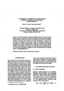
optimally as possible. These maps can be constructed from engineering expertise and insight, or using more formal methods such as optimization [17] or fuzzy logic [18-19]. Stochastic dynamic programming (SDP) methods are particularly appealing in this context, despite their well-recognized computational complexity [20], because of their ability to optimize a power split map for a probabilistic distribution of many drive cycles, rather than a single cycle [21-25]. The above survey briefly examines the hybrid power management literature for both plug-in and conventional hybrid electric vehicles. Within the specific context of PHEVs, power management research has generally focused on fuel economy improvement, subject to constraints on battery state of charge, using either the rule-based [16,17] or DDP approach [9,10]. This paper extends this research by adding three important original contributions to the PHEV power management literature. First, it uses SDP to optimize PHEV power management over a probability distribution of drive cycles. Second, it explicitly accounts for the interplay between fuel and electricity costs in PHEV power management. This makes it possible, for the first time, to fully explore the potential benefits of controlled charge depletion over aggressive charge depletion followed by charge sustenance. Finally, the paper presents what the authors believe to be the first study on the impact of variable electricity and petroleum purchase prices on optimal PHEV power management. The above contributions are made specifically for a single-mode power-split PHEV configuration, although the paper’s approach is extendible to other configurations as well. The remainder of this paper is organized as follows: Section 2 introduces the vehicle configuration, problem definition, and vehicle model used in this work. Section 3 then describes the numerical optimization method adopted in this work. Section 4 discusses the results of this optimization, and Section 5 highlights the paper’s key conclusions. 2. PROBLEM FORMULATION Figure 1 portrays the main components and configuration of the powertrain architecture considered in this paper, often called the single-mode power split, “series/parallel”, or “combined”. This architecture combines internal combustion engine power with power from two electric motor/generators – identified as M/G1 and M/G2 – through a planetary gear set. The planetary gear set creates both series and parallel paths for power flow to the wheels. The parallel flow paths (blue arrows) include a path from the engine to the wheels and a path from the battery, through the motors, to the wheels. The series flow path, on the other hand, takes power from the engine to the battery first, then back through the electrical system to the wheels (red arrows). This redundancy of power flow paths, together with battery storage capacity, increases the degree to which one can optimize powertrain control for performance and efficiency while meeting overall vehicle power demand.
FIGURE 1. SINGLE MODE POWER-SPLIT HYBRID ARCHITECTURE (ADAPTED FROM [26]).
The above power split hybrid vehicle architecture can be used for a variety of vehicle sizes and needs. This paper focuses on a midsize sedan power split PHEV whose key component sizes are listed in Table 1. This PHEV is quite similar in configuration, dynamics, and design to the 2002 Toyota Prius, but with roughly twice the battery capacity. Specifically, we assume that the PHEV has 80 modules of Ni-MH batteries instead of 38 in the 2002 Prius. This choice of battery size and type is partly motivated by the relative ease with which one can convert the above conventional hybrid vehicle into an experimental PHEV – by simply adding Ni-MH battery energy capacity. A subsequent paper builds on this paper’s results by examining the influence of battery sizing on the optimal control laws studied herein [27]. Furthermore, the impact of battery type (e.g., Lithium-ion vs. NiMH, etc.) on PHEV performance and efficiency is the subject of ongoing research that also builds on the methods and results of this paper. Given the above vehicle, powertrain, and battery choices, this paper examines the following power management problem: Minimize:
Subject to:
N −1 J = lim E ∑ γ k g ( x ( k ) , u ( k ) ) N →∞ Pdem k =0 x ( k + 1) = f ( x ( k ) , u ( k ) ) x∈ X
(1)
(2)
u ∈U In this discrete-time stochastic optimal control problem, k represents an arbitrary discrete time instant, and the sampling time is 1 second. This sampling time is consistent with the paper’s focus on supervisory, rather than servo-, control. The optimization objective in this control problem consists of the instantaneous combined cost of PHEV fuel and electricity consumption, g(x(k),u(k)), accumulated over time, discounted by a
TABLE 1. POWERTRAIN MODEL SPECIFICATIONS
Vehicle
EPA Classification Base Curb Weight
Midsize sedan 1400 kg
Engine
Type Displacement Max. Power Max. Torque
Gasoline Inline 4-cylinder 1.5 L 43 kW @ 4000 RPM 102 N-m @ 4000 RPM
Motor/ Generators
Battery Pack
Type Permanent Magnet AC M/G1 Max. Power 15 kW @ 3000-5500 RPM M/G2 Max. Power 33 kW @ 1040-5600 RPM Cell Chemistry Nominal Voltage Nominal Capacity No. of Cells Pack Energy Capacity
Nickel Metal Hydride 1.2 V per cell 6.0 A-h per cell 480 3.7 kWh
constant factor γ, and averaged over the stochastic distribution of instantaneous power demand, Pdem. In optimizing this objective, we impose three important constraints, namely, (i) the PHEV powertrain’s dynamics, represented by f(x(k),u(k)), (ii) the set of admissible PHEV states, X, and (iii) the set of admissible control inputs, U. The remainder of this section presents these optimization objectives and constraints in more detail. Specifically, Sections 2.1-2.4 present, respectively, the PHEV model, f(x(k),u(k)), the optimization functional g(x(k),u(k)), the state and control constraint sets, X and U, and the Markov chainbased drive cycle model used for computing the expected PHEV optimization cost. 2.1 PHEV Model To model the dynamics of a PHEV, we first identify the PHEV’s inputs, outputs, and state variables. Towards this goal, Figure 2 presents a conceptual map of the key interactions between the PHEV examined in this paper, its human driver, and its supervisory power management algorithm. This conceptual map adopts the fairly common tradition in hybrid power management research of interpreting the driver’s accelerator and brake pedal positions as a power signal, Pdem, demanded at the wheels (e.g., [22-24]). The supervisory power management algorithm attempts to meet this power demand by adjusting three control input signals: engine torque Te, M/G1 torque TM/G1, and M/G2 torque TM/G2. Engine startup and shutdown can also be treated as a control input, but this paper assumes, for simplicity, that the PHEV engine idles when power is not demanded. This leaves the important issue of engine startup/shutdown, and its complex impact on PHEV warmup and emissions, as open topics for ongoing research. In summary, therefore, the PHEV plant has three control inputs, namely, the three engine/motor/generator torques.
FIGURE 2. PHEV MODEL COMPONENTS AND CONTROL SIGNAL FLOW.
The above control inputs affect the PHEV plant by affecting its state variables. In this paper, we closely follow some of the existing hybrid vehicle power management research by choosing engine crankshaft speed, ωe, longitudinal vehicle velocity, v, and battery state of charge, SOC, as the three PHEV state variables. We use a Markov memory variable to represent the stochastic distribution of driver power demand, as explained in Section 2.4. To model the dynamics governing the PHEV state variables, we begin by expressing the total road load, Froad, acting on the PHEV as follows [23]:
Froad = Froll + Fdrag + Fdamp ,
(3)
In this equation, Froll is a rolling resistance term given by:
Froll = µ mg ,
(4)
where g, m, and µ represent the acceleration of gravity, mass of the PHEV, and a rolling resistance coefficient (assumed constant), respectively. Furthermore, Fdrag is an aerodynamic drag force given by:
Fdrag = 0.5ρ A fr Cd v 2 ,
(5)
where ρ, Afr and Cd represent the density of air, the PHEV’s effective frontal area, and the PHEV’s effective aerodynamic drag coefficient, respectively. Finally, Fdamp is a wheel/axle bearing friction term given by:
Fdamp =
bw v , rtire
(6)
where bw is the bearing’s damping coefficient and rtire is an effective PHEV tire radius. Note that this expression for wheel
Tring = TM / G 2 ωring = ωM / G 2
damping, as well as other derivations below, assumes a direct proportionality between wheel angular velocity and vehicle speed, where the proportionality constant is related to the tire radius and final drive ratio. This assumption effectively neglects tire slip for simplicity, thereby eliminating the need for using two separate state variables to represent wheel and vehicle speeds. Road loads from Eq. (3) act on the PHEV powertrain through the planetary gear set sketched in Fig. 3. This planetary gear set can be conceptually and mathematically treated as an ideal “lever” connecting the engine, two motor/generators, and vehicle wheels (through the final drive), as shown in Fig. 3. Using this lever diagram in conjunction with Euler’s equations of motion, one can relate the road load in Eq. (3) to angular velocities in the PHEV powertrain as follows [23]:
Ie 0 0 I M / G1 0 0 S − ( R + S )
0 0 I M′ / G 2 R
R + S ωɺ e Te − S ωɺ M / G1 TM / G1 (7) = − R ωɺ M / G 2 TM′ / G 2 0 F 0
In this equation, R and S denote the numbers of teeth on the planetary gear set’s ring and sun, respectively. The angular velocities of the engine and two motor/generators are denoted by ωe, ωM/G1, and ωM/G2, respectively. Furthermore, Te and Ie denote the engine’s brake torque and inertia, and TM/G1 and IM/G1 denote the torque and inertia of the first motor/generator, respectively. The force F represents an internal reaction force between the planetary gear set’s sun and planets. Finally, the terms I’M/G2 and T’M/G2 are effective inertia and torque terms given by: 2 I M′ / G 2 = I M / G 2 + ( I w + mrtire )/ K2
TM′ / G 2 = TM / G 2 − Froad rtire / K
Tcarrier = Te ωcarrier = ωe
Tsun = TM / G1 ωsun = ωM / G1 FIGURE 3. PLANETARY GEAR SET & LEVER DIAGRAM.
To complete the derivation of the PHEV plant model, we assume – for simplicity – that the PHEV’s battery can be idealized as an open-circuit voltage, Voc, in series with some internal resistance, Rbatt. We allow both Voc and Rbatt to depend on battery state-of-charge, SOC, through a predefined map (adapted from [28,29]). Furthermore, we define SOC as the ratio of charge stored in the battery to some known maximum charge capacity, Qbatt. This furnishes the following relationship between the rate of change of SOC and the current, Ibatt, generated by the battery:
ɺ =−I SOC batt Qbatt
(9)
To obtain an expression for the current, Ibatt, we note that the instantaneous power delivered by the battery to the two motor/generators, Pbatt, is related to Ibatt through the following power balance: 2 Pbatt = Voc I batt − Rbatt I batt
,
(10)
(8) Solving Eq. (9,10) for the rate of change of SOC gives:
where IM/G2 and Iw are the rotational inertias of the second motor/generator and wheel, K is the final drive gear ratio, and TM/G2 is the torque produced by the second motor/generator. The point-mass model in Eq. (7,8) provides a complete description of how the state variables ωe and v (which is directly proportional to ωM/G2) evolve with time for given control input trajectories. This description is provided in differential algebraic equation (DAE) form, with the force F and velocity ωM/G1 acting as dependent state variables. Simple algebraic manipulations, omitted herein, can be used in conjunction with time discretization to convert this DAE description to the explicit form in Eq. (2).
2 ɺ = − Voc − Voc − 4 Pbatt Rbatt SOC 2Qbatt Rbatt
(11)
Finally, relating the power Pbatt to the torques, speeds, and efficiencies of the two motor/generators gives:
Pbatt = TM /G1 ω M /G1 η MM/G/G11 + TM /G 2 ω M /G 2 η MM/G/G 22
(12)
−1, Tiωi > 0 for i = {M / G1, M / G 2} ki = 1, Tiωi ≤ 0
(13)
k
where
k
Combining Eq. (11-13) with maps from [28], which relate the efficiencies of the electric motor/generators to their torques and speeds, provides a complete description of the battery SOC dynamics as a function of PHEV states and inputs. Discretizing this description and combining it with an explicit discretized form
of Eq. (7,8) furnishes a complete model of the PHEV plant dynamics, i.e., f(x(k),u(k)) in Eq. (2). This model mostly replicates existing hybrid powertrain models in the literature (e.g., [23]), but we use it in conjunction with the novel objective function in Section 2.2 to examine PHEV power management. 2.2 Objective Function The optimization objective, J, in Eq. (1) aggregates the expected combined cost of PHEV fuel and electricity consumption over a stochastic distribution of trips, and discounts this cost exponentially through the factor γ. This discount factor, if restricted to the interval [0,1), ensures that the cumulative optimization objective remains finite over infinite time horizons. This paper follows Lin [22] in setting γ to 0.95, leaving the question of how different values of γ affect optimal PHEV power management open for future research. To explicitly trade off fuel and electricity consumption in PHEVs, we define the instantaneous cost functional, namely, g(x(k),u(k)) in Eq. (1), as follows:
g ( x, u ) = βα fuelW fuel + α elec
1
η grid
Pelec
(14)
The first term in this cost functional quantifies PHEV fuel consumption, while the second term quantifies electricity consumption, and the coefficient β makes it possible to carefully study tradeoffs between the two. Specifically, Wfuel represents the fuel consumption rate in grams per time step, where we use the engine map in [28] to convert engine torque and speed to fuel consumption. The constant parameter αfuel then converts this rate to an energy consumption rate, in megajoules (MJ) per time step. Similarly, Pelec represents the instantaneous rate of change of the battery’s internal energy, i.e., i
Pelec = −Voc Qbatt SOC
(15)
The constant parameter αelec converts Pelec to MJ per time step. Dividing this change in stored battery energy by a constant charging efficiency ηgrid = 0.98 (which corresponds to a full recharge in six hours) furnishes an estimate of the amount of energy needed from the grid to replenish the battery. Note that Pelec is positive when the PHEV uses stored battery energy and negative during regeneration. Hence, there exists a reward for regeneration that offsets the need to consume grid electricity. The magnitude of this reward depends on the parameter β , which represents the relative price of gasoline per MJ to the price of grid electricity per MJ. We refer to this parameter as the “energy price ratio,” and use it to examine the tradeoffs between fuel consumption and electricity consumption in PHEVs. Specifically, we begin this paper’s power management optimization studies by setting a price ratio of β = 0.8, consistent with the average energy
prices in 2006, namely $2.64 USD per gallon of gasoline and $0.089 USD per kWh of electricity [30]. We then vary this ratio to examine the influence of different relative fuel-to-electricity prices on optimal power management, as shown in Section 4.3. 2.3 Constraints In optimizing PHEV power management, we seek controllers capable of keeping the state vector x within simple bounds expressed as a constraint set X in Eq. (16). These bounds ensure that the engine neither exceeds its maximum allowable speed nor falls to speeds where noise, vibrations, and harshness (NVH) become excessive [26]. They also constrain battery state of charge to remain between two limits denoted as SOCmin = 0.25 and SOCmax = 0.9. Constraining SOC in such a way helps to protect against capacity and power fade due to over-charging or excessive discharging [10,16,17]. However, the precise impact of the depths and rates of PHEV battery charging/discharging on battery health is still under investigation. Finally, we also impose limits on the speeds of the motor/generators to protect them from damage. As explained in Section 3.2, when solving the optimal PHEV power management problem numerically, we use penalty functions to implement all of these state constraints as “soft” constraints.
ωe ,min ≤ ωe ≤ ωe ,max ω ω ω ≤ ≤ M / G1 M / G1,max X = x : M / G1,min ωM / G 2,min ≤ ωM / G 2 ≤ ωM / G 2,max SOCmin ≤ SOC ≤ SOCmax
(16)
In addition to constraining the PHEV state variables, we also implement two types of control input constraints as part of power management optimization: a drivability constraint and control input bounds. The drivability constraint, given by Eq. (17), ensures that driver power demand is met by equating it to the sum of the three engine/motor/generator power outputs:
Pdem = Pe + PM / G1 + PM / G 2
(17)
Since the power output of each PHEV actuator equals its torque multiplied by its angular velocity, which depends directly on the PHEV’s states, this constraint reduces the number of independent control inputs from three to two. The choice of which two torque commands to make independent is arbitrary, but we select engine torque and M/G1 torque to match existing work [23]. Hence, the vector of independent control inputs becomes:
u = [Te
TM / G1 ]
T
(18)
As with the state variables, we constrain the two elements of this vector to take values within an admissible control set denoted by U(x) in Eq. (19). This control set limits the rate of battery charging and discharging to minimize battery damage, and also limits the engine and motor/generator torque to safe and attainable
values. We refer to control policies that map states to control inputs within this set as “admissible” policies [20].
Te ,min ≤ Te ≤ Te ,max (ωe ) TM / G1,min ≤ TM / G1 ≤ TM / G1,max (ωM / G1 ) U ( x ) = u : TM / G 2,min ≤ TM / G 2 ≤ TM / G 2,max (ωM / G 2 ) Pchg ,lim ( SOC ) ≤ Pbatt ≤ Pdis ,lim ( SOC )
(19)
2.4 Drive Cycle Modeling The drive cycle model is a stochastic component to the plant model which predicts the distribution of future power demands using a discrete-time Markov chain [31]. Specifically, the model defines a probability of reaching a certain power demand in the next time step, given the power demand and vehicle speed in the current time step [22]. To acquire a numerical realization of this model, we define a state space for the Markov chain by selecting a finite number of power demand and vehicle speed samples. Then we form an array of conditional transition probabilities according to:
pi , j , m = Pr ( Pdem ( k + 1) = i | Pdem ( k ) = j , v ( k ) = m )
(20)
where i,j index power demand and m indexes vehicle speed. To estimate these transition probabilities, one needs observation data for both power demand and vehicle speed. We obtain these observations from a number of drive cycle profiles. The profiles provide histories of vehicle speed versus time, and we invert the PHEV dynamics to extract corresponding power demand histories. This results in the following equation for power demand, solely in terms of vehicle velocity and vehicle parameters:
Pdem = m
dv 1 v + ρ A fr C d v 3 + µ mgv + bw v 2 rtire dt 2
(21)
In this work, we used federal drive cycles (FTP-72, US06, HWFET) and real-world micro trips (WVUCITY, WVUSUB, WVUINTER) in the ADVISOR database [28] to compute the observation data. We then derived the transition probabilities in Eq. (20) from this data using maximum likelihood estimation [32]. 3. STOCHASTIC DYNAMIC PROGRAMMING This section presents the stochastic dynamic programming approach used for solving the optimal power management problem posed in Section 2. The approach begins with a uniform discretization of the admissible state and control input sets, X and U(x). This discretization makes the optimal power management problem amenable to computer calculations, but generally produces suboptimal results. We use the symbols X and U(x) to refer to both the continuous and discrete-valued state and control input sets for ease of reading. Given the discrete-valued sets, we apply a modified policy iteration algorithm [20] to compute the optimal power management cost function and policy. This algorithm consists of two successive steps, namely, policy
evaluation and policy improvement, repeated iteratively until convergence. For each possible PHEV state, the policy iteration step approximates the corresponding “cost-to-go”, J, which may be intuitively interpreted as the expected cost function value averaged over a stochastic distribution of drive cycles starting at that state. The policy improvement step then approximates the optimal control policy, u*, corresponding to each possible PHEV state. This process iterates, as shown in Fig. 4, until convergence. Sections 3.1 and 3.2 present the policy iteration and policy improvement steps in further detail. 3.1 Policy Evaluation The policy evaluation step computes the cost-to-go for each state vector value, x, given a control policy, u(x). This computation is performed recursively as shown in Eq. (22):
J n +1 ( x ) = g ( x, u ) +
E γ J n ( f ( x, u ) )
∀x ∈ X
Pdem
(22)
The index n in the above recurrence relation represents an iteration number, and the recurrence relation is evaluated iteratively for all state vector values in the discretized set of admissible states, X. In general, the cost-to-go values within the expectation operator must be interpolated because f(x,u) will not always generate values in the discrete-valued state set X. Although the true cost-to-go for a given control policy must satisfy Jn = Jn+1, we iterate Eq. (22) a finite number of times before executing the policy improvement step (next section). This truncated policy evaluation approach, used in combination with the policy improvement step below, converges to the optimal control policy regardless of the maximum number of iterations [20]. 3.2 Policy Improvement Bellman’s principle of optimality indicates that the optimal control policy for the stochastic dynamic programming problem in Eq. (1,2) is also the control policy that minimizes the cost-to-go function J(x) in Eq. (22). Thus, to find this control policy u*, we minimize cost-to-go with respect to this policy for each state vector value x, given the cost-to-go function J(x). Mathematically, this minimization is represented by:
{
}
u * ( x ) = arg min g ( x, u ) + E γ J ( x ) + g cons ( x ) Pdem u∈U ( x )
∀x ∈ X (23)
Equation (23) imposes the state and control input set constraints from Eq. (2) in the form of a quadratic penalty term, gcons(x). This penalty term consists of sixteen penalty functions summed together, each corresponding to one of the inequalities given in Eq. (16) and Eq. (19). Each penalty function equals the excursion from the corresponding constraint boundary, normalized with respect to the feasible range of operation, squared, and multiplied by a coefficient five orders of magnitude greater than the energy
consumption weights. For example, the penalty function for minimum engine speed takes the form:
g cons ,ωe ,min ( x ) = α cons ,ωe ,min
ωe ,min − ωe min 0, ωe,max − ωe ,min
2
(24)
After both policy evaluation and policy improvement are completed, the optimal control policy is passed back into the policy evaluation step and the entire procedure is repeated iteratively. The process terminates when the infinity norm of the difference between two consecutive steps is less than 1%, for both the cost and control functions.
4.1 Performance To illustrate the potential performance improvements of a blending strategy over a CDCS strategy, consider their responses for two FTP-72 drive cycles simulated back-to-back, as shown in Fig. 5 and 6. The total cost of energy for this trip is 6.4% less for the blended strategy relative to CDCS, and fuel consumption is reduced by 8.2%. Blending accomplishes this by utilizing the engine more during the charge depletion phase, thereby assisting the battery to meet total power demand more often than CDCS. Although in the blended case the engine operates at higher loads, therefore consuming more fuel, the engine efficiency is greater and, as demonstrated in Fig. 6, battery charge depletes more slowly. As a result, blending and CDCS incur nearly the same total energy costs through the depletion phase (Fig. 5), and the advantage of blending in terms of overall cost arises from its delayed entry into charge sustenance. 0.9
FIGURE 4: MODIFIED POLICY ITERATION FLOWCHART.
0.7
Cost (USD)
0.6 0.5 0.4 0.3 0.2 0.1 0
0
500
1000
1500
2000
2500
Time (sec)
FIGURE 5. ENERGY CONSUMPTION COSTS, 2X FTP-72. 1 Blended CDCS
0.9 0.8 0.7 SOC
4. RESULTS AND DISCUSSION This section analyzes the properties of the proposed PHEV power management approach by comparing its performance against a baseline control policy, inspired by previous research [1,16,17]. Specifically, it is fairly common in PHEV power management research to examine algorithms that initially operate in a charge depletion mode, then switch to charge sustenance once some minimal battery state of charge is reached [1,16,17]. The charge depletion mode typically utilizes stored battery energy to meet as much of the driver power demand as possible (engine power may be needed when demand exceeds the power capabilities of the motor/generators), thereby depleting battery charge rapidly. The charge sustenance mode then uses engine power to regulate battery state of charge once it reaches some predefined minimum. This charge depletion, charge sustenance (CDCS) approach implicitly assumes that fuel consumption dominates operating costs relative to electricity consumption from the battery. We implement CDCS in this paper by setting αelec in Eq. (14) to zero and rely on the minimum SOC constraint in Eq. (16) to enforce charge sustenance behavior once battery charge is depleted. We refer to power management strategies that are the result of setting all coefficients in Eq. (14) to nonzero values as blended, since a weighted sum of both electricity and fuel is utilized to construct the power split map.
Blended: Total Cost Blended: Fuel Cost Blended: Elec Cost CDCS: Total Cost CDCS: Fuel Cost CDCS: Elec Cost
0.8
0.6 0.5 0.4 0.3
In the remainder of this section, we first analyze the performance of the blended and CDCS strategies by focusing on two FTP-72 drive cycles simulated back-to-back. Second, we examine the difference between these two control strategies in more depth by exploring how they manage engine speed and torque. Finally, we investigate the impact of varying fuel and electricity purchase prices on the optimal blended and CDCS control laws.
0.2
0
500
1000
1500 Time (sec)
2000
2500
FIGURE 6. SOC RESPONSE, 2X FTP-72.
The benefit of delayed entry into charge sustenance is evident from previous research in the literature in which the PHEV drive cycle and total trip length were assumed to be known a priori (e.g., [9,16]). For example, in [9] deterministic dynamic
Performance improvements of blending over CDCS are uniform across all the drive cycles shown in Table 2, where the drive cycle lengths are selected to ensure that the vehicle reaches charge sustenance before the trip terminates. If the vehicle reaches its destination before entering charge sustenance phase, however, the total energy consumption costs are nearly identical for blending and CDCS (as demonstrated in Fig. 5). Therefore the blending strategy proposed herein has no significant energy consumption cost penalty for early trip termination. Note that some of the largest improvements are observed for drive cycles that were not used to estimate the Markov state transition probability matrix.
when the electric machines saturate and cannot meet driver power demand by themselves. This limits the control authority of the electric machines when driver power demand is large, thereby reducing their ability to move engine speed to the optimal operating line. These observations explain how the blending strategy utilizes the engine and electric motors more efficiently, thereby delaying the charge sustenance phase and improving overall PHEV operating costs. 100
20 0
225
80 70
0 25
60 25 0
km/USD
MJ/km
2xFTP-72
8.2%
6.4%
5.4%
US06
3.2%
2.8%
3.2%
4xSC03
11.8%
8.8%
7.7%
HWFET
8.7%
4.9%
4.9%
LA92
11.0%
6.7%
5.9%
25 0
25 0
50 40
27 5
30
30 0
20
32 5 35 0 400
10
600
27 5
275
0 1000
Fuel Economy
BSFC (g/kW*hr) Optimal Op. Pts. Blended Op. Pts.
225
TABLE 2. BLENDED PERFORMANCE IMPROVEMENT OVER CDCS
Drive Cycle
22 5
20 0
90
Torque (N*m)
programming furnished blending strategies that reached minimum SOC exactly when the PHEV trip terminated, thereby never allowing the PHEV to enter the charge sustenance mode. This result agrees with our current findings, namely, that the primary benefit of blending strategies results from their ability to delay or eliminate the need for charge sustenance. However, the approach in [9] requires knowledge of trip length a priori. Since SDP explicitly takes into account a probability distribution of drive cycle behavior, our identified strategy is optimal in the average sense.
300 325 350 400
450 500 550 650 700 800
1500
600
2000
30 0 32 5 35 0 400
450 500 550 650 700 800
2500 Speed (RPM)
600
3000
4000
FIGURE 7. BLENDED OPERATING POINTS ON BSFC MAP, 2X FTP-72. 100
20 0
22 5
90 20 0 225
BSFC (g/kW*hr) Optimal Op. Pts. CDCS Op. Pts.
80 225
Torque (N*m)
70
4.2 Engine Control A significant benefit of the power-split architecture is the fact that it decouples the engine crankshaft from the road, and allows the electric machines to move engine speed where fuel efficiency is maximized [26]. This optimal operating line is identified by the black dashed line in Fig. 7 and 8. As shown in Fig. 7, the blending strategy initially operates the engine at fairly low speeds and high torques, close to the optimal fuel efficiency operating line. This occurs even when power demand can be met by the electric motors alone. The excess engine power goes towards regenerating battery charge, which the blended cost function in Eq. (14) rewards. Moreover, the electric machines are not generally saturated and are thus free to maintain low engine speeds and high efficiencies. In contrast, the CDCS strategy causes the engine to remain at very low brake torque levels during depletion, where fuel consumption is low but so is engine efficiency (Fig. 8). Moreover, significant power is requested from the engine only
450 5000 55 650 7000 80 90 0 3500
60 25 0
40 30 20 10 0 1000
25 0
25 0
50
450 500 550 600
1500
27 5
27 5
27 5
30 0
30 0
325 35 0 400
450 500 550 600
650 700 800
2000
325 350 400
32 5 35 0 40 0
450 500 0 55 600
650 700 800
2500 Speed (RPM)
30 0
3000
6500 70 80 0 90 0 3500
4000
FIGURE 8. CDCS OPERATING POINTS ON BSFC MAP, 2X FTP-72.
4.3 Energy Price Ratio An important feature of the proposed power management algorithm is its dependence on the energy price ratio, β , which varies temporally (e.g., by year) and spatially (e.g., by geographic region). To investigate the nature of this dependence, we obtained
the history of energy price ratios since 1973 [30], shown in Fig. 9. The value of β has clearly changed significantly over the past 35 years due to shifts in both oil and electricity prices. This motivates the need to understand how this parameter impacts optimal PHEV power management.
demand when conventional generation is scarce [33]. This suggests that, with the appropriate exchange of information, a vehicle could be configured to modify its control policy in real time to reflect grid conditions. Hence, our proposed controller is extendible toward vehicle-to-grid infrastructures.
1
Energy Price Ratio, β
0.9 0.8 0.7 0.6 0.5 0.4 1970
1975
1980
1985
1990 Year
1995
2000
2005
2010
FIGURE 9. HISTORIC ENERGY PRICE RATIO DATA.
Consider the SOC depletion responses shown in Fig. 10 for controllers synthesized with energy price ratios in the set β∈{0.4,0.6,0.8,1.0,1.2} and for a CDCS strategy, which by definition does not depend on β . Several conclusions can be drawn from this parametric study. First, as β approaches infinity (i.e. fuel becomes infinitely more expensive than grid electric energy), the optimal blending strategy converges to a CDCS strategy. This is consistent with the fact that the CDCS strategy implicitly assumes the cost of fuel is infinitely more than the cost of electricity. Secondly, for sufficiently low β (i.e. electricity becomes more expensive than fuel), the optimal blending strategy generates electric energy. The implicit assumption leading to this result is that the driver is able to sell energy back to the grid when the vehicle is plugged in. Although electricity prices are unlikely to be this high in general, real-time pricing could motivate using the vehicle as a distributed power generator during periods of peak 1
0.8 0.7
SOC
6. REFERENCES [1] Shabashevich, A., Saucedo, D., Williams, T., Reif, C., Lattoraca, C., Jungers, B., Wietzel, B., Frank, A. A., 2007, “Consumer Ready Plug-in Hybrid Electric Vehicle,” TeamFate, University of California, Davis. http://www.teamfate.net/technical/UCDavis_Spring2007_TechReport.pdf. [2] Ronning, J. J., 1997, “The Viable Environmental Car: the Right Combination of Electrical and Combustion Energy for Transportation,” SAE Papers Number 971629. [3] Simpson, A., 2006, "Cost-Benefit Analysis of Plug-in Hybrid Electric Vehicle Technology," 22nd International Battery, Hybrid and Fuel Cell Electric Vehicle Symposium and Exhibition (EVS-22), Yokohama, Japan. [4] Paganelli, G., Ercole, G., Brahma, A., 2001, "General Supervisory Control Policy for the Energy Optimization of Charge-Sustaining Hybrid Electric Vehicles," JSAE Review, 22(4) pp. 511-518.
0.9
[5] Musardo, C., Rizzoni, G., Guezennec, Y., 2005, "A-ECMS: An Adaptive Algorithm for Hybrid Electric Vehicle Energy Management," European Journal of Control, 11(4-5) pp. 509-524.
0.6
β β β β β
0.5 0.4 0.3 0.2
5. CONCLUSIONS This paper demonstrates the use of stochastic dynamic programming for optimal PHEV power management. It derives an optimal power management strategy that rations battery charge by blending engine and battery power in a manner that improves engine efficiency and reduces total charge sustenance time. This strategy explicitly takes into account a probability distribution of drive cycles and variable energy price ratios. This formulation guarantees a solution that is optimal in the average sense, without requiring drive cycle knowledge a priori. Moreover, we have shown that energy price ratios can significantly influence the characteristics of the optimal control policy. Indeed, it may be useful to equip production PHEVs with a range of control laws corresponding to the range of price ratios that could be experienced over the life of the vehicle.
= 0.4 = 0.6 = 0.8 = 1.0
= 1.2 CDCS 0
500
1000
1500
2000
2500
Time (sec)
FIGURE 10. SOC RESPONSES FOR BLENDED WITH VARYING β AND CDCS, 2X FTP-72.
[6] Sciarretta, A., Back, M., and Guzzella, L., 2004, "Optimal Control of Parallel Hybrid Electric Vehicles," IEEE Trans.s on Control Systems Technology, 12(3) pp. 352-63. [7] Brahma, A., Guezennec, Y., and Rizzoni, G., 2000, "Optimal Energy Management in Series Hybrid Electric vehicles," Proc. of 2000 American Control Conference, Chicago, IL, 1, pp. 60-64.
[8] Lin, C.-C., Peng, H., Grizzle, J. W., 2003, "Power Management Strategy for a Parallel Hybrid Electric Truck," IEEE Transactions on Control Systems Technology, 11(6) pp. 839-49. [9] O’Keefe, M. P., Markel, T., 2006, “Dynamic Programming Applied to Investigate Energy Management Strategies for a Plug-in HEV,” Report Number NREL/CP-540-40376, National Renewable Energy Laboratory, Golden, CO. [10] Gong, Q., Li, Y. and Peng, Z.-R., 2007, “Optimal Power Management of Plug-in Hybrid Electric Vehicles with Intelligent Transportation Systems”. Proc of 2007 Int. Conf. on Advanced Intelligent Mech., Zurich, Switzerland, pp. 1-6. [11] Koot, M., Kessels, J. T. B. A., de Jager, B., 2005, "Energy Management Strategies for Vehicular Electric Power Systems," IEEE Transactions on Vehicular Technology, 54(3) pp. 771-782. [12] Vahidi, A., Stefanopoulou, A., and Peng, H., 2006, "Current Management in a Hybrid Fuel Cell Power System: A ModelPredictive Control Approach," IEEE Transactions on Control Systems Technology, 14(6) pp. 1047-1057. [13] Powell, B. K., Bailey, K. E., Cikanek, S. R., 1998, “Dynamic Modeling and Control of Hybrid Electric Vehicle Powertrain System,” IEEE Control Systems Magazine, 18(5), pp. 17-33. [14] Kimura, A., Abe, T., and Sasaki, S., 1999, "Drive Force Control of a Parallel-Series Hybrid System," JSAE Review, 20(3) pp. 337-341. [15] Rizoulis, D., Burl, J., and Beard, J., 2001, “Control Strategies for a Series-Parallel Hybrid Electric Vehicle,” SAE Paper 2001-01-1354.
Assessment and Calibration: Stochastic Dynamic Programming Approach,” Proc. of 2002 American Control Conference, Anchorage, AK, 2, pp. 1425-1430. [22] Lin, C.-C., 2004, “Modeling and control Strategy Development for Hybrid Vehicles,” Ph.D. thesis, University of Michigan, Ann Arbor, MI. [23] Liu, J. and Peng, H, “Modeling and Control of a Power-Split Hybrid Vehicle,” IEEE Transactions on Control Systems Technology, Accepted for future publiciation. [24] Tate, E., 2007, “Techniques for Hybrid Electric Vehicle Controller Synthesis,” Ph.D. thesis, University of Michigan, Ann Arbor, MI. [25] Johannesson, L., Asbogard, M., and Egardt, B., 2007, "Assessing the Potential of Predictive Control for Hybrid Vehicle Powertrains using Stochastic Dynamic Programming," IEEE Transactions on Intelligent Transportation Systems, 8(1) pp. 71-83. [26] K. Muta, M. Yamazaki, J. Tokieda, “Development of NewGeneration Hybrid System THS II – Drastic Improvement of Power Performance and Fuel Economy,” SAE Papers 200401-0064, 2004. [27] Moura, S. J., Callaway, D. S., Fathy, H. K., Stein, J. L, 2008, “Impact of Battery Sizing on Stochastic Optimal Power Management in Plug-in Hybrid Electric Vehicles”. To appear in Proceedings of 2008 International Conference on Vehicular Electronics and Safety, Columbus, Ohio, USA. [28] Wipke, K. B., Cuddy, M. R., and Burch, S. D., 1999, "ADVISOR 2.1: A User-Friendly Advanced Powertrain Simulation using a Combined Backward/Forward Approach," IEEE Transactions on Vehicular Technology, 48(6) pp. 17511761.
[16] Sharer, P. B., Rousseau, A., Karbowski, D., 2008, "Plug-in Hybrid Electric Vehicle Control Strategy: Comparison between EV and Charge-Depleting Options," SAE Paper 2008-01-0460, 2008 SAE World Congress.
[29] Johnson, V. H., 2002, "Battery Performance Models in ADVISOR," Journal of Power Sources, 110(2) pp. 321-329.
[17] Rousseau, A., Pagerit, S., and Gao, D., 2007, "Plug-in Hybrid Electric Vehicle Control Strategy Parameter Optimization," Electric Vehicle Symposium-23, Anaheim, CA.
[30] Anonymous, 2007, “Annual Energy Review,” U.S. Department of Energy, Tech. Rep. DOE/EIA-0384(2006), URL: http://www.eia.doe.gov/aer/
[18] Schouten, N. J., Salman, M. A., and Kheir, N. A., 2002, "Fuzzy Logic Control for Parallel Hybrid Vehicles," IEEE Transactions on Control Systems Technology, 10(3) pp. 4608.
[31] Gubner, J. A., 2006, Probability and Random Processes for Electrical and Computer Engineers, Cambridge University Press, New York, NY, Chap. 12.
[19] Baumann, B. M., Washington, G., Glenn, B. C., 2000, "Mechatronic Design and Control of Hybrid Electric Vehicles," IEEE/ASME Transactions on Mechatronics, 5(1) pp. 58-72. [20] Bertsekas, D., 1995, Dynamic Programming and Optimal Control: Vol. 2, Athena Scientific, Belmont, MA, Chap. 1. [21] Kolmanovsky, I., Siverguina, I., Lygoe, B., 2002, “Optimization of Powertrain Operating Policy for Feasibility
[32] Anderson, T. W., and Goodman, L. A., 1957, "Statistical Inference about Markov Chains," Annals of Mathematical Statistics, 28(1) pp. 89-110. [33] Kempton, W., Tomić, J., 2005, “Vehicle-to-Grid Power Fundamentals: Calculating Capacity and New Revenue,” Journal of Power Sources, 144(1), pp. 268-278.