for compressing neural spike data. ... SNR of the spike data apart from having a compression ratio of 150 : 1. ... in online spike compression for BMI applications.
A Novel Weighted LBG Algorithm for Neural Spike Compression Sudhir Rao, Ant´onio R. C. Paiva, Jos´e C. Pr´ıncipe Abstract— In this paper, we present a weighted Linde-BuzoGray algorithm (WLBG) as a powerful and efficient technique for compressing neural spike data. We compare this technique with the recently proposed Self-Organizing Map with Dynamic Learning (SOM-DL) and the traditional SOM. A significant achievement of WLBG over SOM-DL is a 15dB increase in the SNR of the spike data apart from having a compression ratio of 150 : 1. Being simple and extremely fast, this algorithm allows real-time implementation on DSP chips opening new opportunities in BMI applications.
I. I NTRODUCTION Brain Machine Interfaces (BMI) aim at establishing a direct communication pathway between human or animal brain and external devices (prosthetics, computers) [1]. The ultimate goal is to provide paralysed or motor-impaired patients a mode of communication through the translation of thought into direct computer control. In this emerging technology, a tiny chip containing hundreds of electrodes are chronically implanted in the motor, premotor and parietal cortices and connected through wires to external signal processor which is then processed to generate control signals [2], [3]. Recently, attempts to develop wireless neuronal data transmission protocols has gained considerable attention [4]. Not only would this enable increased mobility and reduce risk of infection in clinical settings, but also would free cumbersome wired behavior paradigms where experimenter must overcome issues like entanglement, torque applied to prosthetics and chewing of cables. Although this idea looks simple, a major bottleneck in implementing it is the high constraints on the bandwidth and power imposed on these bio-chips. On the other hand, to extract as much information as possible we would like to transmit all the electrophysiological signals for which the bandwidth requirement can be daunting. For example, to transmit the entire raw digitized potentials from 32 channels sampled at 20kHz with 16 bits of resolution we need a huge bandwidth of 10Mbps. Many solutions were proposed to solve this problem. One solution is to perform spike detection on site, and then transmit spike signal only or the time at which the spike occurred [5]. An alternative is to use spike detection and sorting techniques so that binning (the number of spikes in a given time interval) can be immediately done [4]. The disadvantage of these methods lies in the weakness of current automated spike detection methods without human interaction as well as the missed opportunities of any post processing since the original waveform is lost. It is in this regard, that we propose The authors are with the Computational Neuroengineering Laboratory (CNEL), Department of Electrical and Computer Engineering, University of Florida, Gainesville, FL 32611, USA (phone: 352-392-2682; fax: 352392-0044; email: {sudhir,arpaiva,principe}@cnel.ufl.edu).
to compress the raw neuron potentials using well established vector quantization techniques. The goal of vector quantization is efficient and compact representation of data with few codewords. The most common method of doing vector quantization (VQ) is to minimize a distortion measure between the set of codewords and the data. k-means and LBG [6] are the two most popular VQ algorithms which achieve this by minimizing the L2 norm. Another popular and widely used technique is Kohonen’s self organizing maps (SOM) [7] which not only represents the data efficiently but also preserves the topology by a process of competition and cooperation between neurons. In fact, self organizing maps without lateral interactions between neurons are standard vector quantizers [8]. Paiva et al. [9] successfully trained SOM on the neural data recordings. The strategy was to transmit through the wireless link only the index determined by the SOM, which encodes the raw digitized potentials. As with any common vector quantization technique, this would represent the dense region very well and use few code vectors for sparse regions. Unfortunately, this means poor encoding of spikes which are generally sparse in the neural recordings. To correct this, a new algorithm called self organizing map with dynamic learning (SOM-DL) was introduced [10]. Though there is slight improvement in the SNR of the spike region, the changes made were heuristic. Further, these algorithms are computationally intensive with large number of parameters to tune and can only be executed offline. In this paper, we introduce a new weighted LBG (WLBG) algorithm which effectively solves this problem. Using a novel weighting factor we give more weightage to sparse region corresponding to the spikes in the neural data leading to a 15dB increase in the SNR of the spike region. The simplicity and the speed of the algorithm makes it feasible to implement this in real-time opening new doors of opportunity in online spike compression for BMI applications. In the next section we give a brief overview of our algorithm and SOM-DL. Section 3 deals with details of the neural data. The novel waiting factor is introduced in section 4. Finally, we present our results in section 5 and conclude in section 6. II. T HEORY The WLBG is actually a recursive implementation of weighted k-means algorithm. The cost function optimized is the weighted L2 distortion measure between the data points and the codebook as shown below in (2). D(C) =
N ∑ i=1
wi kxi − c∗i k , 2
(2)
Step 1 Specify the maximum distortion allow Dmax and maximum number of levels Lmax . Step 2 Initialize L = 0 and codebook C as random point in Rd . Step 3 Set M = 2L . Start the optimization loop a. Calculate for each xi ∈ X, the nearest code vector c∗i ∈ C using (3). b. Update the the code vectors in the codebook using (1) where the sum is taken over all data points for which cj is the nearest code vector. ∑ k:c∗ =cj wk xk (1) cj = ∑ k k:c∗ =cj wk k
c. Measure the new distortion D(C) as shown in (2). If D(C) ≤ Dmax then go to step 5 or else continue. d. Go back to (a) unless the change in distortion measure is less than δ Step 4 If L = Lmax , go to step 5 . Else L = L + 1 and split each point cj ∈ C into two point cj + ² and cj − ² and go back to step 3. Step 5 Stop the algorithm. Return C, the optimized codebook. Fig. 1.
The outline of WLBG algorithm.
where c∗i is the nearest code vector to data point xi as given in (3). 2 c∗i = min kxi − cj k (3) cj ∈C
d Consider a dataset X = (xi )N i=1 ∈ R . Let C = (cj )M denote the codebook to be found. The outline of j=1 the algorithm is show in Fig. 1. Both δ and ² are set to a very small value. A typical value is δ = 0.001 and ² = 0.0001[1 − 1 − 1 . . .] where the random 1 and -1 is a d dimensional vector. This recursive splitting of the codebook has two advantages over the direct k-means method. 1) Firstly, there is no need to specify the exact number of code vectors. In most real applications, the maximum distortion level Dmax is known. The LBG algorithm starts with one code vector and recursively splits it so that D(C) ≤ Dmax . 2) Secondly, the recursive splitting effectively avoids the formation of empty clusters which is very common in k-means.
A. SOM and SOM-DL Self organizing maps (SOM) is an idea based on competitive learning. The goal is to learn the non linear mapping between the data in the input space and a two or one dimensional fully connected lattice of neurons in an adaptive and topologically ordered fashion [11]. Each processing element (PE) in the lattice of M PEs has a corresponding synaptic weight vector which has the same dimensionality as that of the input space. At every iteration, the synaptic weight closest to every input vector xk is found as shown in (4). i∗ = argmin kxk − wi k (4) 1≤i≤M
Having found the winner PE for each xk , a topological neighborhood is determined around the winner neuron. The weight vector of each PE is then updated as wi,k+1 = wi,k + ηk Λi,k (xk − wi,k ),
(5)
where ηk ∈ [0, 1] is the learning rate. The topological neigh( 2) i∗ k borhood is typically defined as Λi,k = exp − kri −r 2 2σk where kri − ri∗ k represents the Euclidean distance in the output lattice between ith PE and the winner PE. Notice that both learning rate (ηk ) and the neighborhood width (σk ) are time dependent and are normally annealed for best performance. When applying SOM to neural data it was found that most of the PEs were used to model the noise rather than the spikes in the data. This is typical of any neural recording which generally has sparse number of spikes. In order to alleviate this problem and to move PEs from low amplitude region of state space to the one corresponding to the spikes the following update rule was proposed. wi,k+1 = wi,k + µΛi,k sign(xk − wi,k )(xk − wi,k )2
(6)
This was called self organizing map with dynamic learning (SOM-DL) [10]. By accelerating the movements of the PEs toward the spikes, the SOM-DL represents the spikes better. But for good performance careful tuning of the parameters is important. For example, it was experimentally verified that µ between 0.05 and 0.5 balances between fast convergence and small quantization error for the spikes. Further, it is well known that SOM based algorithms are computationally very intensive. III. N EURAL DATA We test this algorithm on synthetic neural data which was designed to emulate as accurately as possible the scenario encountered with actual recordings of neuronal activity. The waveform contains spike from two neurons differing in both peak amplitude and width as shown in Fig. 2(a). Both neurons fired according to homogeneous Poisson process with firing rates of 10 spikes/s (continuous line) and 20 spikes/s (dotted line). Further, to introduce some variability in the recorded template each time a neuron fired the template was scaled by a Gaussian distributed random number with
1.2
1.2 spike1 spike2
1
1 0.8
0.8
0.6 0.6 0.4 0.4 0.2 0.2 0 0
−0.2
−0.2 −0.4
−0.4
0
5
10
15
20
25
30
(a) Spikes from two different neurons
−0.6 −0.6
−0.4
−0.2
0
0.2
0.4
0.6
0.8
1
1.2
Fig. 3. 2-D embedding of training data which consists of total 100 spikes with a certain ratio of spikes from the two different neurons
1.2 1
Thus, we select the weighting for our algorithm as shown below { 2 2 kxi k if kxi k ≥ τ wi = (7) 2 τ if kxi k ≤ τ ,
0.8 0.6 0.4 0.2 0 −0.2 −0.4 −0.6 4.4
4.5
4.6
4.7
4.8
4.9 4
x 10
(b) An instance of the neural data Fig. 2.
Neural Dataset and the waveforms of the two neurons
mean 1 and standard deviation 0.01. Finally, the waveform was contaminated with zero mean white noise of standard deviation 0.05. An instance of the neural data is shown in Fig. 2(b). IV. N OVEL W EIGHTING FACTOR Since we are interested in the reconstruction of spikes as accurately as possible, a separate training dataset was constructed with 100 spikes as if they had been segmented from a real waveform after spike detection. A two dimensional non overlapping embedding of the training data is shown in Fig. 3. Since the spikes correspond to large amplitudes in magnitude, the farther the data point from the origin the more likely it is to belong to the spike region. Further, information at the tip of the spike should be modeled well since amplitude of the spike is an important feature in spike sorting. Thus, to reconstruct spike information as accurately as possible we need to give more weightage to the points far from the origin.
where τ is a small constant to prevent the weighting from going to zero. Though an arbitrary choice of τ would do, we can make an intelligent selection. Note that we can estimate the standard deviation σ of the noise from the data which corresponds to the dense gaussian cluster at the origin in Fig. 3. Since 2σ denotes 95 percent confidence interval of the gaussian noise, therefore we can set τ = (2σ)2 giving same weightage to all points belonging to the gaussian noise. In our experiment σ = 0.05 and so we set τ = 0.01. V. R ESULTS In this section, we present the results obtained by WLBG on the neural spike data using the novel weighting factor developed in previous section and compare it with results obtained from SOM-DL and SOM. Fig. 4 shows 16 point quantization obtained using WLBG on the training data. As can be seen more code vectors are used to model the points far away from the origin even though they are sparse. This helps to code the spike information in greater details and hence minimize reconstruction errors. On the other hand, SOM-DL wastes a lot of points in modeling the noise cluster as shown in Fig. 5. Further, not only does SOM-DL have large number of parameters which needs to be fine tuned for optimal performance, but also takes immense amount of time to train the network making it only suitable for off line training. We test this on a separate test data generated to emulate real neural spike signal. A small region is highlighted in Fig. 6 which shows the comparison between the original and the reconstructed signal. Clearly WLBG does a very good job in preserving spike features. Also notice the suppression of noise in the non-spike region. This denoising ability is
1.2
data
1
1
reconstructed
0.8 0.6
0.8
0.4
0.6
0.2 0
0.4
−0.2
0.2
−0.4
0
2.226
2.227
2.228
2.229
2.23
2.231
2.232
2.233
2.234 4
x 10
−0.2 −0.4
Fig. 6. Performance of WLBG in reconstructing spike regions in test data −0.6 −0.6
−0.4
−0.2
0
0.2
0.4
0.6
0.8
1
1.2
TABLE I SNR Fig. 4.
OF SPIKE REGION AND THE WHOLE TEST DATA OBTAINED USING
16 point quantization of training data using WLBG
WLBG, SOM-DL SNR of Spike region Whole test data
1
WLBG 31.12dB 8.12dB
AND
SOM
SOM-DL 16.53dB 8.97dB
SOM 14.7dB 10.08dB
0.8 0.6
sampled at 20kHz and digitized to 16 bits of resolution. We use this to measure the firing rate of the code vectors. Fig. 7 shows the probability of firing of the WLBG codebook. Code vector 16 (centered near origin in Fig. 4) models the noisy part of the signal and hence fires most of the time. It should be noted that in general neural data has very sparse number of actual spikes.
0.4 0.2 0 −0.2 −0.4
−0.4
−0.2
0
0.2
0.4
0.6
0.8
1
1.2
1 0.9
Fig. 5. Two-dimensional embedding of training data and quantization vectors in a 5 × 5 lattice trained by SOM-DL.
0.8 0.7 0.6
one of the strengths of this algorithms and is attributed to the novel weighting factor we selected. We report the SNR obtained by using WLBG, SOMDL and SOM in Table I. As can be seen, there is a huge increase of 15dB in the SNR of the spike regions of the test data compared to SOM-DL which only marginally improves the SNR over SOM. Obviously, by concentrating more on the spike region, our performance on the non-spike region suffers but the decrease is negligible compared to SOMDL. It should be noted that good reconstruction of the spike region is of utmost importance and hence the only measure which should be considered is the SNR in the spike region. Further, the result reported here for WLBG is for 16 code vectors which is far less than 25 code vectors (5 × 5 lattice) for SOM-DL and SOM algorithms. A. Compression Ratio We quantify here the theoretical compression ratio achievable by using the codebook generated by WLBG. In order to do so, we use a test data consisting of 5 seconds of spike data
0.5 0.4 0.3 0.2 0.1 0
0
Fig. 7.
2
4
6
8
10
12
14
16
Firing probability of WLBG codebook on test data
The probability values for the code vectors is given in Table II. The entropy of this distribution is H(C) =
16 ∑
pi log(pi ) = 0.2141.
i=1
From information theory, we know that this is a lower bound for average number of bits needed to represent the codebook. Thus, with good coding like arithmetic codes we
TABLE II P ROBABILITY VALUES OBTAINED FOR THE CODE VECTORS AND USED IN F IG . 7 Code Vectors 1 2 3 4 5 6 7 8 9 10 11 12 13 14 15 16
Probability 0.0007 0.0017 0.0007 0.0014 0.0003 0.0007 0.0010 0.0193 0.0003 0.0018 0.0007 0.0045 0.0002 0.0015 0.0006 0.9647
can reach very close to this optimal value. Since we are using 2D non overlapping embedding of the signal sampled at 20kHz, the number of bits needed to transmit the data is 20k 2 × 0.2141 = 2.141kbps. If the data had been transmitted without any compression then, the number of bits needed is 20k × 16 = 320kbps. Thus we achieve a compression ratio of 150 and at the same time maintain a 32dB SNR on the spike region. Further, on real datasets, where a 10D embedding is generally used, the compression ratio would increase to 750 with only 428bps needed to transmit the data. This is a significant achievement and would help alleviate the bandwidth problem faced in transmitting data in BMI experiments. VI. C ONCLUSIONS We have proposed a weighted LBG (WLBG) as an excellent compression algorithm for neural spike data with emphasis on good reconstruction of the spikes. The advantages over SOM-DL are apparent but nevertheless listed below. 1) A 15dB increase in SNR of spike regions in the data. 2) A smaller and more efficient codebook achieving a compression ratio of 150 : 1. 3) The increase in speed is many folds. The WLBG takes less than 1 seconds on machine with Pentium IV and 512 MB RAM versus SOM-DL which takes more than 15 minutes. 4) There is no parameters in WLBG compared to SOM algorithms which has step size, neighborhood kernel size and their annealing parameters which needs to be properly tuned. The only variable to be defined in WLBG is the weights wi which have a clear interpretation for the application at hand. 5) Since the WLBG algorithm update just consists of inner products and is extremely fast, it can be easily be implemented in DSP chips for online compression. Future work includes extending this idea to real dataset and constructing an efficient k-d tree search algorithm for the codebook taking into account the weighting factor and
the probability of code vectors. We would also like to use advanced encoding techniques like entropy coding and achieve bit rate as close as possible to the theoretical value. Finally, real-time implementation of this algorithm and applying this to real BMI experiments would also be pursued. ACKNOWLEDGMENT This work was partially supported by NSF grant ECS-0601271 and ECS-0422718. A. R. C. Paiva was supported by Fundac¸a˜ o para a Ciˆencia e a Tecnologia under grant SFRH/BD/18217/2004. The authors would like to thank the anonymous reviewers for their valuable suggestions. R EFERENCES [1] Miguel A. L. Nicolelis, “Brainmachine interfaces to restore motor function and probe neural circuits,” Nature Reviews Neuroscience, vol. 4, pp. 417–422, 2003. [2] Miguel A. L. Nicolelis, Christopher R. Stambaugh, Amy Bristen, and Mark Laubach, “Methods for simultaneous multisite neural ensemble recordings in behaving primates,” in Methods for Neural Ensemble Recordings, Miguel A. L. Nicolelis, Ed., chapter 7, pp. 157–177. CRC Press, 1999. [3] Johan Wessberg, Christopher R. Stambaugh, Jerald D. Kralik, Pamela D. Beck, Mark Laubach, John K. Chapin, Jung Kim, S. James Biggs, Mandayam A. Srinivasan, and Miguel A. L. Nicolelis, “Realtime prediction of hand trajectory by ensembles of cortical neurons in primates,” Nature, vol. 408, no. 6810, pp. 361–365, Nov. 2000. [4] K. D. Wise, D. J. Anderson, J. F. Hetke, D. R. Kipke, and K. Najafi, “Wireless implantable microsystems: high-density electronic interfaces to the nervous system,” Proceedings of the IEEE, vol. 92, no. 1, pp. 76–97, Jan. 2004. [5] Chad A. Bossetti, Jose M Carmena, Miguel A. L. Nicolelis, and Patrick D. Wolf, “Transmission latencies in a telemetry-linked brainmachine interface,” IEEE Transactions on Biomedical Engineering, vol. 51, no. 6, pp. 919–924, June 2004. [6] Y. Linde, Buzo A., and Gray R.M., “An algorithm for vector quantizer design,” IEEE Trans. on Communications, vol. 28, pp. 84–95, Jan. 1980. [7] T. Kohonen, “Self-organized formation of topologically correct feature maps,” Biological Cybernetics, vol. 43, pp. 59–69, 1982. [8] Tom Heskes, “Self-organizing maps, vector quantization, and mixture modeling,” IEEE Transactions on Neural Networks, vol. 12, no. 6, pp. 1299–1305, Nov. 2001. [9] Ant´onio R. C. Paiva, Jos´e C. Pr´ıncipe, and Justin C. Sanchez, “Compression of spike data using the self-organizing map,” in Proc. 2nd Int. IEEE-EMBS Conf. on Neural Engineering, Arlington, VA, Mar. 2005, pp. 233–236. [10] Jeongho Cho, Ant´onio R. C. Paiva, Sung-Phil Kim, Justin C. Sanchez, and Jos´e C. Pr´ıncipe, “Self-organizing maps with dynamic learning for signal reconstruction,” Neural Networks, 2007, accepted. [11] S. Haykin, Neural Networks: A Comprehensive Foundation, 2nd edition, New Jersey, Prentice Hall, 1999.