A p-norm Flow Optimization Problem in Dense Wireless ... - CiteSeerX

A p-norm Flow Optimization Problem in Dense Wireless Sensor Networks Mehdi Kalantari, Masoumeh Haghpanahi, Mark Shayman Department of Electrical and Computer Engineering, University of Maryland {mehkalan, masoumeh, shayman}@eng.umd.edu

Abstract— In a network with a high density of wireless nodes, we model flow of information by a continuous vector field known as the information flow vector field. We use a mathematical model that translates a communication network composed of a large but finite number of sensors into a continuum of nodes on which information flow is formulated by a vector field. The magnitude of this vector field is the intensity of the communication activity, and its orientation is the direction in which the traffic is forwarded. The information flow vector field satisfies a set of Neumann boundary conditions and a partial differential equation (PDE) involving the divergence of information, but the divergence constraint and Neumann boundary conditions do not specify the information flow vector field uniquely, and leave us freedom to optimize certain measures within their feasible set. Therefore, we introduce a p-norm flow optimization problem in which we minimize the p-norm of information flow vector field over the area of the network. This problem is a convex optimization problem, and we use sequential quadratic programming (SQP) to solve it. SQP is known for numerical stability and fast convergence to the optimal solution in convex optimization problems. By using standard SQP on p-norm flow optimization, we prove that the solution of each iteration of SQP is uniquely specified by an elliptic PDE with generalized Neumann boundary conditions. The p-norm flow optimization shows interesting properties for different values of p. For example, if p is close to one, the information routes resemble the geometric shortest paths of the sources and sinks, and for p = 2, the information flow shows an analogy to electrostatics. For infinitely large values of p, the problem minimizes the maximum magnitude of the information vector field over the network, and hence it achieves maximum load balancing.

I. I NTRODUCTION Wireless sensor networks have been a subject of interest of many researchers in recent years. Fast growth of microelectronics and microprocessing devices have resulted in devices with very small physical dimensions and a small per sensor cost. The small cost of the devices enables networks with several hundred to several thousand sensors distributed in a geographical area. There are many applications for such networks including military, environment monitoring, transportation systems, surveillance, agriculture and home applications. Generally, sensors use radio frequency channels for communicating, and it is desired to collect the data acquired by all sensors in one or a few specific destinations in the network for processing. Such stations are known as sinks or fusion centers. For communicating with the traffic sinks, the sensors relay the packets of each other in a multi-hop way. This work was partially supported by AFOSR under grant F496200210217 and NSF under grants CNS-0519554 and CCF-0729129.

As the number of wireless nodes grow, careful analysis of the network behavior becomes very hard by using conventional methods that employ a discrete model in space. In discrete models, different network properties such as transport rate of information are only evaluated at the locations of the wireless nodes. A main shortcoming of discrete models is that often the flow models become computationally prohibitive when the number of wireless nodes grows very large. We use a continuous space model to formulate flow of information in a wireless network with a large number of nodes. For this purpose, we use a vector field model that represents flow of information at every point of a network. We introduced this idea in our former work [1,2], with a model inspired by electrostatics and using analogy of propagation of an electric field in a dielectric media with information transport in a network. In those works we used a quadratic cost function, and showed that solution to the optimization problem is found by solving a set of PDEs analogous to Maxwell’s equations in electrostatics. Our work was followed by Toumpis and Tassiulas [3,4], where the authors showed that minimizing the quadratic cost function results in optimal deployment of sensors by minimizing the number of sensor nodes required to transport all the information to the intended sinks. In a recent work [5], we have given an optimization for the case that there are multiple commodity flows in the network, and we need to make a joint optimization on multiple flows. In this methodology an information flow vector field models transportation of traffic in a wireless network. The vector field has two components at every location of the network: a magnitude that represents the density of communication at that location and an orientation that gives the direction to which the traffic is forwarded. The model is most suitable in situations where the sensors in the network are distributed with a high enough density so that the routes from individual sensors to the traffic sinks can be chosen to well approximate the flux lines of the vector field passing through the sensors. The first property of the vector field is that it satisfies a partial differential equation (PDE), which impose the constraint that the traffic of all sources should be routed to their destinations. This constraint is incorporated into our model through the divergence of the vector field and represents flow conservation in conventional networks. Additionally, the vector field satisfies a set of Neumann boundary conditions, which state that the vector field has a zero component in the direction normal to the boundary of the network.

We present a general method for flow optimization in a wireless sensor network. In this method, we minimize a pnorm of the information flow vector field subject to the basic flow constraints (i.e., flow conservation and boundary constraints). We have called this problem the p-norm flow optimization. In this problem we always have p > 1. The pnorm optimization problem has several interesting properties for different values of p. For example, when p is close to 1, the routes tend to pass through shortest geometric paths from a source to a sink, and as a result the average transport delay is less compared to the case with higher values of p. When p is close to 1, the optimization does not make the best use of network resources, and for example, it may leave a lot of resources unused while some areas of the network that lie on shortest paths are overloaded by the network traffic. By increasing the value of p from 1 the optimization tries to spread the traffic in the network and use the resources more evenly. While this increases delay, it helps load balance the traffic compared to the case where p is smaller. The limiting case of p → ∞ is a minmax problem, where the maximum magnitude of the information flow vector field is minimized. Load balancing can be beneficial in numerous ways such as increasing the transport capacity of the network by using standard techniques such as spatial multiplexing and uniform use of network resources such as the nodes’ batteries. While the case p → ∞ achieves maximal load balancing, it may use longer paths for some portions of the traffic. In practical applications, p can be selected based on a trade-off between delay and balancing the traffic over the network. In order to solve the p-norm flow optimization, we first show that this problem is a convex optimization problem. Then, we use Sequential Quadratic Programming (SQP) to solve the pnorm flow optimization on a general network geometry. SQP uses iterations, and in each iteration, it finds the quadratic approximation of the optimization problem around an operating point and solves the resulting quadratic optimization problem. Then it adds the solution to the operating point and finds a new operating point and repeats iterations. SQP is known for numerical stability and fast convergence to the optimal solution in convex optimization problems. We prove that the solution to each iteration of SQP is uniquely specified by an elliptic PDE with generalized Neumann boundary conditions. This elliptic PDE has a standard canonical form. There are several lines of works that have studied dense wireless sensor networks. Non-quadratic cost functions in the flow problem were considered in [4], where the authors considered a general form of cost function, and optimizing the cost function requires solving nonlinear PDEs. Such PDEs are hard to solve for a generic cost function. Additionally, properties of the solutions for general cost functions are unknown. In comparison to the cost functions in [4], the p-norm flow optimization is a less general form of the cost function, but we present a concrete method to solve the resulting PDEs and give an in depth insight into the properties of the solution for different values of p. Load balancing problem in dense wireless sensor networks was studied in [6]. In this work,

the authors consider a minmax optimization problem and develop lower bounds for the objective of the achievable minimum. In [7], the performance of load balancing methods in the presence of multipath routes were compared with single path approaches, and it was shown that under certain models, the performance of the multipath approach does not give significant improvement unless the number of paths between a source and a destination is large enough. In [8], the analogy between information paths in a dense ad hoc network and light paths in optics was studied, and it was shown that the routes bend when the spatial density of nodes change in the network. This analogy was studied in further detail in [9], where the approach was developed for wireless networks with energy and bandwidth constraints. The asymptotic capacity of wireless networks in the number of nodes was studied in [10]. Our approach is distinguished from the body of existing work in two aspects: (i) We introduce p-norm as a family of optimization problems for a wireless sensor network in a general network geometry that is densely covered by sensors, where varying p results in different properties in the information flow. (ii) We use SQP to solve the p-norm problem and show that the solution to each iteration of SQP is uniquely defined by an elliptic PDE. The remainder of this paper is organized as follows: First we introduce the basic definitions and notations in Section II. In Section III we give a brief background on formulating information flow as a vector field and discuss the solutions in the case where we minimize a quadratic cost function. In Section IV we introduce the p-norm flow optimization problem and use SQP to solve this problem. We show how the solution to each iteration of SQP is found by solving an elliptic PDE. An illustrative numerical example is given in Section V, and we conclude the paper in Section VI. II. N OTATIONS AND DEFINITIONS In this section, we give a brief summary of our notations and definitions. To avoid confusion, we only introduce notations that we will use frequently. There are other symbols and notations that we will introduce where they are first used. Throughout this paper, boldface characters represent vector quantities. We use z = (x, y) to represents location in R2 . Unless we state otherwise, we use Cartesian coordinate system to express vector quantities, where ˆi and ˆj represent the unit vectors along x and y axes, respectively. For a generic vector quantity we use the notation v = (vx , vy ) to represent the vector, where vx and vy are the x and y components of v in a Cartesian coordinate system. Whenever we need to manipulate a vector as a matrix, we consider the vector as a 2 × 1 matrix: v = [vx vy ]T . In order to make PDE expressions simpler, we use the nabla ∂ˆ ∂ ˆ i + ∂y j; for a vector quantity F = (Fx , Fy ), operator: ∇ = ∂x the density of sources of the vector field is found by the divergence of F, which is defined as ∇·F=

∂Fy ∂Fx + ∂x ∂y

Similarly, ∇×F represents the density of rotation of F, which is expressed as: ∇ × F = (−

∂Fy ˆ ∂Fx + )k ∂y ∂x

ˆ = ˆi × ˆj. in which k For a scalar function u(z), we use ∇u to represent the gradient of u. Moreover, we use the Laplacian operator, ∇2 , which appears in the form of Poisson equation in information flow in the case of quadratic optimization: ∇2 u =

2

2

∂ u ∂ u + 2 ∂x2 ∂y

The network is located in a closed, connected, and bounded set A ∈ R2 . The information sources are distributed with a spatial density function µ(z) ∈ A, which means that at location z = (x, y) ∈ A, µs (z) bps/m2 of information is generated. The information of the sources is needed to be transported to a set of distributed sinks. The sinks are distributed according to a density function µd (z) bps/m2 . The total information generated by the sources is equal to
µ (z)dxdy = the total information collected by the sinks: A s
µ (z)dxdy. Based on the above notions, we define the A d generalized density of information sources ρ(z) = µs (z) − µd (z) . Since all the
information of sources is transported to the sinks, we have A ρ(z)dxdy = 0. The p-norm of an n × 1 vector X = (x1 , x2 , · · · , xN ) is: N  p1  |X|p = |xi |p i=1

Similarly, the p-norm of function f (z) where f : A → R is:   p1 p |f |p = |f (z)| dxdy A

For a scalar function u(z), where u : A → R, the PDE c11

∂2u ∂2u ∂2u ∂u ∂u + c + b2 =g + 2c + b1 12 22 ∂x2 ∂x∂y ∂y 2 ∂x ∂y

is the canonical form of a general second order linear PDE on A. In the above PDE c11 , c12 , c22 , b1 , b2 , and g are A → R functions. The above PDE is an elliptic PDE if the following matrix is positive semidefinite for every point z ∈ A:  c11 c12 C= c12 c22 III. BACKGROUND : INFORMATION FLOW AS A VECTOR FIELD

In this section, we give a brief overview of our previous work on routing in wireless networks by using vector fields. We briefly state our results here; more complete presentations of these results can be found in [1,2,11]. In the first step, we define a vector quantity that models flow of information. Let D(z) = (Dx , Dy ) denote this vector field whose direction represents the direction of flow of information at point z, and its magnitude represents the density

of information rate passing per unit length of a line segment perpendicular to the direction of D(z). In other words, if we consider a line segment with a small length ∆ at z and perpendicular to the direction of D(z), the information crosses that line segment with rate |D(z)|∆. The above definition of D(z) implies that for a closed contour C ∈ A we have: 

D(z) · dn = ρ(z)dxdy (1) C

S(C)

in which dn is a differential vector normal to the contour at each point of its boundary and pointing to the outside of the contour, the dot represents the inner product of vectors in two-dimensional space, and S(C) is the area surrounded by the closed contour C. Equation (1) is analogous to Gauss’ law in electrostatics theory, and it has a simple interpretation in our formulation: the rate at which information exits a contour is the net sum of the sources inside that contour. The following is known as the Divergence Theorem in vector calculus: 

∂Dy ∂Dx + )dxdy (2) D · dn = ( ∂y C S(C) ∂x Equations (1) and (2) hold for an arbitrary contour C. This implies the following PDE form for information flow: ∇ · D(z) =

∂Dx ∂Dy + = ρ(z) ∂x ∂y

(3)

It is important to note that (3) is a representation of the flow conservation law in continuous form. The boundary condition of the above PDE is a result of the fact that information is not intended to exit the boundary of the network or enter it from the outside. Hence: Dn (z) = 0, z ∈ ∂A

(4)

in which Dn (z) is the normal component of D(z) on the boundary of A, and ∂A represents the boundary of A. This condition is known as Neumann boundary condition. An important note about PDE (3) with the boundary condition (4) is that these equations do not result in a unique value for D(z). Therefore, we have freedom to impose additional condition(s) to optimize D(z) such that the resulting vector field generates a desirable property. In [1,2] we introduced a quadratic cost function of the information flow vector field D in order to find a unique solution:  |D(z)|2 dxdy (5) Minimize J(D) = A

s.t.

∇ · D(z) = ρ(z) Dn (z) = 0, z ∈ ∂A

The above form of cost function results in spatial spreading of the communication load over the space available in the network. To some extent, it balances the communication load of the network in such a way that it avoids having a high load somewhere in the network while the resources are underutilized somewhere else. Moreover, it is shown in [3] that minimizing the cost function in (5) minimizes the number

of sensor nodes required to handle the total communication burden of the network. Our former result shows that the cost function in (5) is optimal if and only if the curl of D(z) is zero: ∇ × D(z) = (−

∂Dy ˆ ∂Dx + )k = 0 ∂y ∂x

Since ∇×D = 0, then D is conservative, and it can be written as the gradient of a scalar potential function: D(z) = ∇U (z). This potential function satisfies the Poisson’s equation: ∇2 U (z) =

∂2U ∂2U + = ρ(z) 2 ∂x ∂y 2

(6)

IV. p-norm FLOW OPTIMIZATION PROBLEM One of the main motivations for using a quadratic cost function is to disperse the traffic in the network. By spreading the communication load of the network over the space, we make the best use of the available resources in the network. This reduces the interference among the wireless nodes, and increases the overall network throughput. However, the quadratic cost function does not achieve maximum spatial spreading of the traffic over the network. In this section, we consider the following general form of optimization problem:  |D(z)|p dxdy Minimize J(D) = A

∇ · D(z) = ρ(z) Dn (z) = 0, z ∈ ∂A

A

∇ · D(z) = ρ(z) Dn (z) = 0, z ∈ ∂A

˜ J(D) = (max |D(z)|) z∈A

∇ · D(z) = ρ(z) Dn (z) = 0, z ∈ ∂A

which is a minmax problem and minimizes the maximum value of |D(z)| over the network area A. Apparently the maximal spatial spreading is achieved in this case, and therefore the corresponding D(z) is a very attractive case for the purpose of balancing the traffic load over the network. Our first observation is that the p-norm flow optimization is a convex optimization problem. Recall that D(z) = (Dx (z), Dy (z)), in which Dx (z) and Dy (z) represent the x and y components of D(z), respectively. Hence, if we define g(Dx , Dy ) = |D(z)|p , the second derivatives of g is:  2  2 H(g) =  p(Dx2

+

∂ g 2 ∂Dx

∂ g ∂Dx ∂Dy

∂2g ∂Dx ∂Dy

∂2g ∂Dy2

p−4 Dy2 ) 2



=

(p − 1)Dx2 + Dy2 (p − 2)Dx Dy

(p − 2)Dx Dy Dx2 + (p − 1)Dy2



(9) in which H(g) is the Hessian of g. Performing the eigenvalue decomposition on H(g) we find:

(7) H(g) =

in which p > 1 is a real number. Recall that the constraints of the above optimization problem ensure delivery of the traffic generated by the sources to the sinks. Note that increasing the value of p causes the optimization problem to increase the amount of spatial spreading in the network. To illustrate this fact consider a point z belonging to an infinitesimal area dS. Since dS is infinitely small, the value of |D(z)| over it is almost constant, and hence the contribution to the cost function due to dS is |D(z)|p |dS|. Now if we double the value of |D(z)|, then the above value of contribution increases by a factor of 2p . This simple observation suggests that by using larger values of p, the optimization problem tends towards solutions that make more spatial spreading, which in turn results in a better spatial diversity of the network. An observation about the optimization (7) is that this problem is equivalent to the case in which we raise the cost function to power 1/p:  p1  p ˜ |D(z)| dxdy (8) Minimize J(D) = s.t.

Minimize s.t.

The combination of the divergence property, the zero-curl property, and the boundary conditions uniquely specify D(z). The boundary conditions of D imply that the partial derivative of U is zero along the normal direction to the boundary of A.

s.t.

Note that the cost function in the recent optimization problem is the p-norm of the information flow vector field D. Based on this observation, we call the optimization (7) the p-norm flow optimization problem. To further illustrate the fact that increasing p results in more spatial spreading, we study the case when p → ∞ in which p-norm gives the maximum absolute value of |D(z)| over the network, and the optimization problem becomes equivalent to:

Dy + Dx (10) Note that the eigenvalues of H(g) are υ1 = p(p − 1)(Dx2 + Dy2 )p/2−1 , and υ2 = p(Dx2 + Dy2 )p/2−1 . Therefore, both eigenvalues are nonnegative, and hence, the matrix H(g) is positive semidefinite, which implies that g is convex in (Dx , Dy ). We observe that the cost function J in p-norm flow optimization (7) is the integral of g over the network area, and the constraints are linear in (Dx , Dy ).

p(Dx2

p−4 Dy2 ) 2



Dx Dy

−Dy Dx



p−1 0

0 1



Dx −Dy

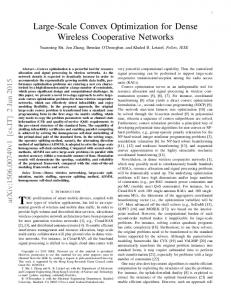
A. An Illustrative Example We study a simple example to illustrate the performance of p-norm flow optimization on a simple network geometry shown in Fig. 1. In this example, a source located on the left hand side of the network generates information at a rate of θ bps. The information of the source needs to be transmitted to a destination on the right hand side of the network as depicted in Fig. 1. There are two geometric paths between the source and the destination. Both paths have equal widths of W , but different lengths denoted by L1 and L2 , respectively. For transporting information from the source to the destination, we assume θ1 bps is transmitted through path 1, and θ2

Fig. 1. Illustrating effect of the p-norm flow optimization. The amount of θ bits/sec traffic of a source is divided between to geometric paths. The paths have different lengths but equal widths. For p → 1 the optimization chooses the shortest path. For p = 2, it splits the traffic such that θ1 L1 = θ2 L2 . For p → ∞, the optimization performs load balancing by setting θ1 = θ2 .

is transmitted through path 2. The information is transported over the two paths by sensors that densely cover the area of both paths and relay packets from the source to the destination. The basic definition of D gives the following magnitude for the information flow vector field on the two paths: θ1 θ2 , |D2 | = W W Note that the simple network geometry in this example implies that the value of |D| remains constant along each path but different for the two paths. The value of the cost function in this example is:  |D(z)|p dxdy J(D) = |D1 | =

A

= |D1 |p W L1 + |D2 |p W L2 = θ1p W 1−p L1 + θ2p W 1−p L2 We assume that the second path is longer than the first path; therefore, L2 = kL1 , where k > 1. Hence: J(D) = W 1−p L1 (θ1p + kθ2p ) Flow conservation in this example translates into the constraint θ1 + θ2 = θ. Forming the Lagrangian function, the optimality condition is found to be: 1

θ1 = k p−1 θ2 which results in the following optimal values for θ1 and θ2 : θ1 =

1

k p−1

1

1+k p−1

θ,

θ2 =

1

1

1+k p−1

θ

Among values of p, there are three cases of special interest: 1 p → 1, p = 2, and p → ∞. For p → 1, we have k p−1 → ∞; hence θ1 = θ, and θ2 = 0. The p-norm optimization problem in this case chooses the shortest path from the source to the destination. While the shortest paths of p  1 result in minimum delay, they do not use all the network resources and as shown in this case, one of the paths between the source and the destination is left completely unused. The next case of interest is p = 2. For this case we find θ1 = kθ2 , or equivalently, θ1 L1 = θ2 L2 . This implies that the optimization uses both paths, and the amount of information that is transported on each path is inversely proportional to the length of that path. In an earlier work, we have shown that in the case of p = 2, the mathematical model of information

flow vector field has a one-to-one analogy with electrostatics [1,2]. Additionally the special case of p = 2 leads to optimal deployment of sensor nodes and requires the minimum number of sensors to transport the traffic of source to the destination [3]. Notice that p = 2 uses both paths, but it does not achieve a complete load balanced solution. The last case of special interest is the asymptotic case of 1 p → ∞. In this case k p−1 → 1; hence, θ1 = θ2 = θ/2. In this case the optimization problem performs maximum load balancing, and the problem minimizes the maximum value of |D| over the network area. As illustrated in this example, the p-norm flow optimization problem represents a family of optimization problems in which the properties of the resulting routes vary significantly by varying the value of p from one extreme to the other. In practical situations, the value of p depends on the specific requirements of each application and the trade-offs between delay and load balancing. In the next step, we use the convexity of the p-norm flow optimization problem to introduce a set of algebraic PDEs that lead us to the optimal solution. B. Solving the p-norm flow optimization problem In order to solve the p-norm flow optimization problem, we use the SQP iterations. Such iterations are well known for their numerical stability and good convergence speed [12,13]. Additionally, since the p-norm flow optimization is a convex optimization problem, the SQP iterations are guarantied to converge to the global optimum [12]. Each iteration of SQP method can be summarized in the following two steps: Quadratic approximation: Having a value for the information flow vector field as an operating point at the ith iteration, denoted by D(i) , which satisfies the set of constraints given by the divergence property and Neumann’s boundary conditions, we find the quadratic approximation of the optimization problem near D(i) . For this purpose, we assume that the operating point D(i) is perturbed by a small variation denoted by e, and hence, we have D = D(i) + e. Then we find the second order approximation of the cost function J(D) with respect to e. Optimization: In this step we find e that minimizes quadratic cost function of the previous step. Convexity of the p-norm flow optimization problem implies that the quadratic cost is convex in e. By using the method of Lagrange multipliers and the geometric interpretation of the divergence property, we show that the optimal e is found by solving an elliptic PDE with generalized Neumann boundary conditions. After solving this PDE, we add the optimal value of e to D(i) and find a new operating point. We repeat the iterations above until a certain stop criterion is satisfied. We now give a mathematical derivation of SQP method in p-norm optimization detail. Assume at the ith (i) (i) iteration D(i) = (Dx , Dy ) is known and satisfies ∇ · D(i) (z) = ρ(z) (i) Dn (z) = 0, z ∈ ∂A

(11)

(i)

in which Dn (z) represents the normal component of the vector field D(i) along the boundary at a point z ∈ ∂A. Then we define e = (ex , ey ) as the variation of the information flow vector field near D(i) : D(z) = D(i) (z) + e(z)

(12)

Since D must satisfy the divergence property and the Neumann boundary conditions of the p-norm flow optimization problem, we have the following constraints on e: ∇ · e(z) = 0 en (z) = 0, z ∈ ∂A

(13)

where en (z) denotes the normal component of e at z ∈ ∂A. To find the second order approximation of J(D) near D(i) , we use the following:   |D|p dxdy = |D(i) + e|p dxdy (14) J(D) = A A  ≈ |D(i) |p dxdy A   1 + eT ∇g(D(i) ) + eT H(g(D(i) ))e dxdy 2 A (i)

(i)

in which ∇g(D ) and H(g(D )) represent the gradient and the Hessian of g(D) = |D|p with respect to D and evaluated at D(i) , respectively. The expression in (14) is the first 3 terms of the Taylor’s series expansion of the function g. In the next step we find the optimal solution of the quadratic approximation of the cost function by optimizing over e subject to the constraints given by (13). The first term in (14) does not depend on e and can be dropped from the optimization cost function. Hence, we have the following optimization problem over e in each iteration of SQP:    1 T (i) T e R + e Qe dxdy Minimize Jq (e) = 2 A s.t. ∇ · e(z) = 0 (15) en (z) = 0, z ∈ ∂A in which R = ∇g(D(i) ) is a 2 × 1 matrix representing the gradient of g, and Q = H(g(D(i) )) is a 2 × 2 matrix (i) representing Hessian of g, and Jq (e) is the cost function in the ith iteration of SQP. Note that both Q and R are functions of z. Recall that convexity of g in D implies that Q is a positive semidefinite matrix, which was shown (10). We now introduce a scheme that converts the quadratic optimization problem into an elliptic PDE. For this purpose, we state the following lemma: Lemma 1: For the optimal solution of the quadratic optimization problem (15) there exists a scalar function λ(z) : A → R that satisfies: ∇λ = Qe + R

(16)

Proof: To prove the lemma, we use the following identities: Identity 1: If v is a scalar function and F is a vector field, then: ∇ · (vF) = v∇ · F + F · ∇v (17)

Identity 2: If A is a region in the plane with boundary ∂A, and F is a vector field on A, then

 ∇ · Fdxdy = F · dn (18) A

∂A

in which dn is the differential vector normal to the boundary of A pointing outward. This identity is the divergence theorem, which we used earlier in a slightly different form in (2). We use the Lagrangian method to prove Lemma 1. Note that for every point z ∈ A, we have ∇ · e(z) = 0. This implies that for each z ∈ A we need to define the Lagrange multiplier λ(z). This results in the following Lagrangian function:     1 λ∇ · edxdy (19) L(e) = eT R + eT Qe dxdy + 2 A A Using Identity 1 for F = e and v = λ gives: ∇ · (λe) = λ∇ · e + e · ∇λ ⇒ λ∇ · e = ∇ · (λe) − e · ∇λ Substituting this expression for λ∇ · e in (19) gives:    1 L(e) = eT R + eT Qe dxdy 2  A ∇ · (λe)dxdy − e · ∇λdxdy + A

(20)

(21)

A

Next we use Identity 2 for F = λe. This identity implies: 

∇ · (λe)dxdy = λe · dn (22) A

∂A

On the other hand, the boundary conditions of e specified in (13) require that the normal component of this vector field on the boundary of A is zero. Therefore, we have e · dn = 0 for every point z ∈ ∂A, which implies that the right hand side of (22) is zero. Hence:  ∇ · (λe)dxdy = 0 (23) A

Substituting the surface integral above in (21) leads us to:    1 L(e) = eT (R − ∇λ) + eT Qe dxdy (24) 2 A Note that we have used e · ∇λ = eT ∇λ. The rest of the proof is based on calculus of variation. In the Lagrangian function (24), we replace e by ˜ e = e + e , where e : A → R2 is a small variation vector field. The Lagrangian function for ˜ e is:    1 T L(˜ e) = e Q˜ e dxdy ˜ eT (R − ∇λ) + ˜ 2 A    1  T  T  = (e + e ) (R − ∇λ) + (e + e ) Q(e + e ) dxdy 2 A Now we use the fact that e is infinitely small; hence, we can ignore the second order terms. By expanding the integrand and

removing second order terms we find:    1 T T L(˜ e) = e (R − ∇λ) + e Qe dxdy 2 A T e (R − ∇λ + Qe) dxdy + A  T = L(e) + e (R − ∇λ + Qe) dxdy (25) A

Hence the variation of Lagrangian is:  T ∆L := L(˜ e) − L(e) = e (R − ∇λ + Qe) dxdy

(26)

A

Optimality of Lagrangian implies that the above variation is zero for every e . Therefore, we can choose e = (R − ∇λ + Qe), where  is an infinitely small positive number. This choice of e implies that (R − ∇λ + Qe) = 0, and hence ∇λ = Qe + R. QED.1 Lemma 1 gives the main key to converting the optimization problem (15) into a partial differential equation. For this purpose, we use Lemma 1 to write e in terms of the Lagrange multiplier λ: e = Q−1 (∇λ − R)

(27)

We will discuss later that in all cases of interest to us, Q is nonsingular; however, it can be ill-conditioned in special situations. We will discuss later in this section how to handle such cases. Next, we use ∇ · e(z) = 0 which is the first optimization constraint in (15). This implies that: ∇ · e = ∇ · (Q−1 (∇λ − R)) = 0

(28)

Equivalently: ∇ · (C∇λ) =  in which: C(z)

= Q−1 (z) :=



c11 (z) c12 (z) c12 (z) c22 (z)

(29)

= ∇ · (Q−1 (z)R(z)) ∂(r1 c11 + r2 c12 ) ∂(r1 c12 + r2 c22 ) + = ∂x ∂y where r1 and r2 denote the entries of the column vector R = [r1 r2 ]T . Since Q is a positive semidefinite matrix, C = Q−1 is also positive definite. It is straightforward to verify that the second order PDE (29) is elliptic. To illustrate this we substitute the value of ∇λ = [∂λ/∂x ∂λ/∂y]T in this PDE: (z)

∇ · (C∇λ) =  ⇒ ∂(c11 ∂λ/∂x+c12 ∂λ/∂y) ∂x

+

∂(c12 ∂λ/∂x+c22 ∂λ/∂y) ∂y

=

1 Lemma 1 can be generalized as follows: consider the optimization:
J(D) = A f (e)dxdy, subject to: ∇ · e(z) = (z), and en (z) = 0 where z ∈ ∂A, and f : R2 → R is a differentiable function. Then the optimiality conditions are: ∂f ∂λ ∂λ ∂f = = and ∂ex ∂x ∂ey ∂y

The proof is similar to the proof of Lemma 1.

which implies: ∂2λ ∂2λ ∂2λ + c + 2c 12 22 ∂x2 ∂x∂y ∂y 2 ∂c12 ∂λ ∂c12 ∂c22 ∂λ ∂c11 + ) +( + ) + ( ∂x ∂y ∂x ∂x ∂y ∂y =  c11

(30)

Equivalently: c11

∂2λ ∂2λ ∂2λ ∂λ ∂λ + c + b2 =  (31) + 2c + b1 12 22 2 2 ∂x ∂x∂y ∂y ∂x ∂y

∂c12 ∂c12 ∂c22 11 where b1 = ( ∂c ∂x + ∂y ), and b2 = ( ∂x + ∂y ). Since C is positive semidefinite on A, the PDE in (31) is elliptic. The final step is to determine the boundary conditions for λ in the elliptic PDE (31). For this purpose, we translate the Neumann boundary conditions of e into the boundary conditions for λ. Note that we have:

e = C(∇λ − R) Hence for a point z ∈ ∂A with outward unit normal vector n ˆ (z) = [nx (z) ny (z)]T , we have: ˆT e = 0 en (z) = 0 ⇒ n T ⇒n ˆ C(∇λ − R) = 0 ˆ T CR ⇒n ˆ T (C∇λ) = n ∂λ ⇒ (nx c11 + ny c12 ) ∂λ ˆ T CR ∂x + (nx c12 + ny c22 ) ∂y = n which is known as the generalized Neumann boundary condition. The existence and uniqueness of the solution of the elliptic PDEs with generalized Neumann boundary condition is a known fact in the context of PDEs [14]. The argument of this section can be summarized in the following theorem: Theorem 1: The solution to each SQP iteration is specified by e = C(∇λ − R), where λ is uniquely specified by the following elliptic PDE c11

∂2λ ∂2λ ∂2λ ∂λ ∂λ + c + b2 =  (32) + 2c + b1 12 22 2 2 ∂x ∂x∂y ∂y ∂x ∂y

with boundary condition ∂λ (nx c11 + ny c12 ) ∂λ ∂x + (nx c12 + ny c22 ) ∂y T =n ˆ CR, z ∈ ∂A

(33)

An important remark is that the matrix Q is positive semidefinite, and it may happen that in some areas of the network, this matrix is close to singular. This may cause problems in the elliptic PDE (29), which involves C = Q−1 . Note that the eigenvalues of Q = H(g) are: υ1 = p(p − 1)(Dx2 + Dy2 )p/2−1 , and υ2 = p(Dx2 + Dy2 )p/2−1 , and hence, C will be illconditioned when p → 1, or (Dx2 + Dy2 ) → 0. Since for all cases where p > 1 the traffic is spread over the network to some extent and in practice, |D| is nonzero for all of such cases; however, the value of |D| can be very small in some areas of the network, which causes numerical instability in SQP. A method to avoid numerical instability in such cases is to replace a close to zero eigenvalue by a very small positive fixed number  whenever Q is close to singular. The

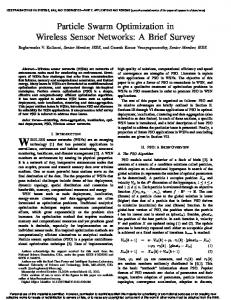
Fig. 2. (a) The information flow vector field for p = 2 used as the initial value of D in SQP iterations. The sources of information are uniformly spread on the two highlighted rectangles and the sink is at the center of the square. (b) Spatial distribution of traffic in the proximity of the sink. The bars show the values of |D| on 12 evenly spaced directions toward the sink and at distance r = 0.2 of the sink. The difference between the maximum and the minimum values of |D| on the 12 directions is 76.88 bps/m.

eigenvalues of Q are lower bounded by  after this correction. Such a correction is standard in SQP when the Hessian matrix is ill-conditioned [12]. In practice the value of  may be very small and for example using a value of  = 10−8 when Q is ill-conditioned has shown good stability in all numerical examples that we have studied. Our final remark is on solving elliptic PDEs in practical applications. Fortunately, the canonic form of the elliptic PDE (32) with the boundary conditions (33) enables us to use the existing powerful numerical PDE solvers. The above elliptic PDE appears in different branches of science and engineering such as electromagnetics, heat exchange, fluid dynamics, and diffusion. Due to the broad spectrum of the applications, the numerical elliptic PDE solvers are very well studied and have reached a high level of accuracy and maturity [14,15]. The solvers use different techniques such as Finite Element Method [15] in order to solve the PDE with a high accuracy in a reasonable time. For example, the Matlab PDE toolbox [16] is capable of solving an elliptic PDE on a square with 64 × 64 grid point in less than one second.2 We need a few SQP iterations to find the solution of the p-norm flow optimization. In all numerical examples that we studied, the SQP shows a fast convergence to the global optima with number of SQP iterations strictly less than 10. V. A N UMERICAL E XAMPLE In this section we present numerical examples that illustrate the performance of p-norm flow optimization with various values of p. Each iteration of SQP requires solving an elliptic PDE for which we have used the PDE toolbox of Matlab3 . We use a network on a 1 × 1 square densely covered by sensors. The network in this scenario is shown in Fig 2. The traffic in this network is generated uniformly inside two equal size rectangles specified by 0.1 ≤ x ≤ 0.2, 0.4 ≤ y ≤ 0.6, and 0.8 ≤ x ≤ 0.9, 0.4 ≤ y ≤ 0.6, respectively. The sources inside the rectangles generate a total of 100 units of traffic. 2 The run time was measured on a generic PC with enough memory and an Intel Pentium IV processor. 3 We have used assempde command to solve the elliptic PDEs. This command solves conic PDEs with canonical form of ∇ · (C∇u) + au = f with Dirichlet, Neumann, or mixed boundary conditions. [16]

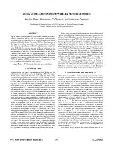
Fig. 3. (a) Information flow vector field after five SQP iterations for p = 8. (b) Spatial distribution of traffic in the proximity of the sink. The bars show values of |D| on 12 evenly spaced directions toward the sink and at distance r = 0.2 of the sink. The difference between the maximum and the minimum values of |D| on the 12 directions is reduced 5.08 bps/m.

Fig. 4. (a) Information flow vector field after six SQP iterations for p = 16. (b) Spatial distribution of traffic in the proximity of the sink. The bars show values of |D| on 12 evenly spaced directions toward the sink and at distance r = 0.2 of the sink. Using p = 16, which is a relatively large value of p, the traffic approaching the sink in different directions is nearly balanced. The difference between the maximum and the minimum values of |D| on the 12 directions is reduced to 2.084 bps/m, which is a steep decrease compared to unbalanced cases such as p = 2.

The traffic of the network is intended to be transported to a sink located at (0.5, 0.5). First, we study the problem with p = 2. In this case the problem is already quadratic, and we do not need SQP to find the optimal D. To find D, we solve the Poisson’s equation given by the PDE (6) for the potential function U with Neumann boundary conditions n ˆ · ∇U = 0. Note that the Poisson’s equation has a simple elliptic form. By taking the gradient of U we compute D. The resulting value of D is shown in Fig. 2-a. The relative size of each arrow reflects the magnitude of D, and its orientation is the direction of D at the corresponding point. In order to show how the traffic approaches the sink, we have plotted the value of |D| on different directions in the proximity of the sink. The plot in Fig. 2-b shows 12 samples of |D| on the perimeter of a small circle with radius r = 0.2 centered at the sink. The horizontal axis of Fig. 2-b shows the angle between 0 and 2π at which each sample on the small circle was taken. As can be seen in this figure, the samples are very uneven, and indeed the difference between the largest and the smallest samples is 76.68 bps/m. An interesting fact about this plot is that the sum of the samples is proportional to the total rate of the traffic being sent to the sink since all the traffic needs to pass the small circle to reach the sink. In the next step we use SQP to solve the p-norm optimization for p = 8. We use the value of D in the previous case

as the initial information flow vector field for SQP iterations, D(0) . The experiments show that after 5 iterations, the SQP converges with a good accuracy (|D(i) −D(i−1) | ≤ 0.1 bps/m). The resulting value of D is shown in Fig. 3-a. As can be seen, the distribution of the traffic changes in the proximity of the sink and the traffic approaches more evenly from the different directions of the sink. This fact is better visualized in Fig. 3-b, where similar to before, we have plotted 12 evenly spaced samples of |D| on the perimeter of a small circle with radius r = 0.2, centered at the sink. In this case, the difference between the largest and the smallest samples reduces to 5.084 bps/m, which shows a steep decrease compared to the case with p = 2. Similarly, for p = 16, the values of D, and the 12 samples of |D| in proximity of the sink are shown in Fig. 4-a and Fig. 4-b, respectively. In this case, the SQP converges after 6 iterations. As can be seen in Fig. 4-b, the pattern of traffic is very uniform in the proximity of sink and the amount of traffic approaching the sink from different directions is almost equal. In this case, the difference between the largest and the smallest samples reduces to 2.084 bps/m. Since p = 16 is a relatively large value of p, the problem has already achieved an almost load balanced solution. Balancing traffic helps the network resources to be utilized in a more even way. Also when the traffic is balanced, we can improve the capacity of the sink (e.g., by spatial multiplexing or space diversity). Since the sink is the major bottleneck of the network, increasing its capacity improves the overall capacity of the network. For example, the sink can use multiple directional antennas to differentiate the signal received on each direction (e.g., 12 identical directional antennas in the case of this example). In such a design, the sink performs a spatial multiplexing on the traffic approaching it in different directions, and therefore, achieving the maximum capacity is only possible when the amount of the traffic received through different directional antennas is balanced. VI. C ONCLUSION In this paper, we presented a family of optimization problems in which the objective is to minimize p-norm of the vector quantity that models flow of information. We use a mathematical model that translates a communication network composed of a large but finite number of sensors into a continuum of nodes on which information flow is formulated by a vector field. The magnitude of this vector field is the intensity of the communication activity, and its orientation is the direction in which the traffic is forwarded. The information flow vector field satisfies a set of Neumann boundary conditions and a PDE involving the divergence of information, but the divergence constraint and Neumann boundary conditions do not specify the information flow vector field uniquely, and leave us freedom to optimize certain measures within their feasible set. In order to solve the p-norm flow optimization problem, we used an SQP method, which is known for fast convergence and good numerical stability in general optimization problems.

We showed that each iteration of SQP for p-norm flow optimization leads us to solving an elliptic PDE with generalized Neumann boundary conditions. Solving the elliptic PDE is easy since this PDE has a canonical form similar to the elliptic PDEs appearing in other branches of science and engineering such as electromagnetics, heat exchange, fluid dynamics, and there are many powerful tools to solve such PDEs with good accuracy and in reasonable time. We showed that the solution of p-norm optimization problem has different properties for different values of p. For example, if p  1, the optimization gives routes that have a tendency to transport the traffic of sources to the sink on the shortest geometrical paths. On the other hand, p → ∞ minimizes the maximum magnitude of the information flow vector field over the network, and therefore, it achieves load balancing. While the solutions for the extreme of p  1 minimize delay, the larger values of p make a more uniform use of the network resources by spreading out the traffic over all possible paths between the sources to the sinks. In practice, the value of p depends on the requirements and the trade-offs between delay and load balancing. R EFERENCES [1] M. Kalantari and M.A. Shayman. Energy efficient routing in sensor networks. In Conference on Information Sciences and Systems, 2004. [2] M. Kalantari and M.A. Shayman. Routing in wireless ad hoc networks by analogy to electrostatic theory. In IEEE International Communications Conference, 2004. [3] S. Toumpis and L. Tassiulas. Efficient node deployment in massively dense sensor networks as an electrostatics problem. In IEEE Infocom, 2005. [4] S. Toumpis and L. Tassiulas. Optimal deployment of large wireless sensor networks. IEEE Transactions on Information Theory, 52(7):2935– 2953, 2006. [5] M. Kalantari and M.A. Shayman. Routing in multi-commodity sensor networks based on partial differential equations. Princeton University, March 2006. [6] Esa Hyytia and Jorma Virtamo. On traffic load distribution and load balancing in densewirelessmultihop networks. EURASIP Journal on Wireless Communications and Networking, 2007, Article ID 1692. [7] Y. Ganjali and A. Keshavarzian. Load balancing in ad hoc networks: single-path routing vs. multi-path routing. In IEEE Infocom 2004. [8] P. Jacquet. Geometry of information propagation in massively dense ad hoc networks. In ACM International Symposium on Mobile Ad Hoc Networking and Computing (MobiHoc 04). [9] S. Toumpis R. Catanuto and G. Morabito. Optic,mal: Optical / optimal routing in massively dense wireless networks. In IEEE Infocom 2007. [10] P. Gupta and P. R. Kumar. The capacity of wireless networks. IEEE Transactions on Information Theory, 46(2):388–404, 2000. [11] M. Kalantari and M.A. Shayman. Design optimization of multisink sensor networks by analogy to electrostatic theory. In Wireless Communication and Networking Conference, 2006. [12] J. Nocedal and S. J. Wright. Numerical Optimization. Springer-Verlag New York, Inc., 1999. [13] S. Boyd and L. Vandenberghe. Convex Optimization. Cambridge University Press, 2003. [14] L. C. Evans. Partial Differential Equations. American Mathematical Society, 1998. [15] G. Haase C. Douglas and U. Langer. A Tutorial on Elliptic PDE Solvers and Their Parallelization. Society for Industrial and Applied Mathematics (SIAM), 2003. [16] The MathWorks. Matlab PDE Toolbox. http://www.mathworks.com/products/pde/.