International Journal of Neural Systems World Scientific Publishing Company
A P300 BRAIN COMPUTER INTERFACE BASED ON A MODIFICATION OF THE MISMATCH NEGATIVITY PARADIGM JING JIN*
Key Laboratory of Advanced Control and Optimization for Chemical Processes, Ministry of Education, East China University of Science and Technology, Shanghai, 200237, China Email:
[email protected] ERIC W SELLERS
Brain-Computer Interface Laboratory, Department of Psychology, East Tennessee State University, 37614 Johnson City, TN, USA Email:
[email protected] SIJIE ZHOU
Key Laboratory of Advanced Control and Optimization for Chemical Processes, Ministry of Education, East China University of Science and Technology, Shanghai, 200237, China Email:
[email protected] YU ZHANG
Key Laboratory of Advanced Control and Optimization for Chemical Processes, Ministry of Education, East China University of Science and Technology, Shanghai, 200237, China Email:
[email protected] XINGYU WANG
Key Laboratory of Advanced Control and Optimization for Chemical Processes, Ministry of Education, East China University of Science and Technology, Shanghai, 200237, China Email:
[email protected] ANDRZEJ CICHOCKI
Laboratory for Advanced Brain Signal Processing, Brain Science Institute, RIKEN, Wako-shi, 351-0198, Japan and Systems Research Institute of Polish Academy of Science, Warsaw, Poland Email:
[email protected] The P300-based brain-computer interface is an extension of the oddball paradigm, and can facilitate communication for people with severe neuromuscular disorders. It has been shown that, In addition to the P300, other ERP components have been shown to contribute to successful operation of the P300 BCI. Incorporating these components into the classification algorithm can improve the classification accuracy and information transfer rate. In this paper, a single character presentation paradigm was compared to a presentation paradigm that is based on the visual mismatch negativity. The mismatch negativity paradigm showed significantly higher classification accuracy and information transfer rates than a single character presentation paradigm. In addition, the mismatch paradigm elicited larger N200 and N400 components than the single character paradigm. The components elicited by the presentation method were consistent with what would be expected from a mismatch paradigm and a typical P300 was also observed. The results show that increasing the signal-to-noise ratio by increasing the amplitude of ERP components can significantly improve BCI speed and accuracy. The mismatch presentation paradigm may be considered a viable option to the traditional P300 BCI paradigm.
*
Corresponding author 1
2
Author’s Names
Keywords: Brain computer interface, Event-related potentials, Mismatch negativity.
1. Introduction Brain computer interface (BCI) technology provides people with a means of communication, or a method to send commands to external devices in real time. Noninvasive BCIs typically rely on the scalp-recorded electroencephalogram (EEG) [1-16]. The P300-based BCI was introduced by Farewell and Donchin (1988) [17]. They showed that the P300 event-related potential (ERP) could be used to successfully select a letter when the subject focused on a target letter and counted how many times the letter flashed. However, it is necessary to average several ERPs for the P300 BCI to obtain high accuracy. The major deleterious side effect of averaging is that it increases the amount of time needed to make a character selection, thereby decreasing information transfer rate (ITR) [18-20]. Many studies have examined ways to improve P300 BCI performance. Several studies have focused on classifier optimization [21-26]. Lenhardt et al., (2008) and Jin et al., (2011b) improved classification accuracy and ITR using strategies that dynamically adapted the number of trials used to make character selections [27, 28]. Zhang at al., (2013) presented spatiotemporal discriminant analysis to decrease the amount of time needed for offline training [31]. In addition, Lu et al., (2009) and Jin et al., (2013) presented generic model strategies that obviated the need for offline training [29, 30]. In addition to classification methods, several studies have focused on reducing the overlap of target epochs and decreasing interference created by items adjacent to the target [27, 32-34]. Target-to-target interval and inter-stimulus interval have also been used to optimize the stimulus sequence [32, 35-38]. In addition to developing new classification methods, novel stimulus presentation paradigms have been proposed. In general, these paradigms have been developed to exploit ERP components in addition to the P300, and to enhance the difference between attended and ignored events. The majority of spatiotemporal features selected by classification algorithms occur at locations and latencies consistent with the P300 [39]. However, stimulus parameters can be manipulated so that additional ERP components will be elicited, and contribute to the classification algorithm. For example, Hong et al., (2009) replaced flashes with motion stimuli that could elicit N200s, which could provide
performance that was superior to a conventional P300 BCI paradigm [40]. Jin et al., (2012) combined motion and flash stimuli, which increased the amplitude of the N200 and P300 components and resulted in higher accuracy and information transfer rate (IRT) [41]. The MMN was first demonstrated by Näätänen et al. (1978) using auditory stimuli [42]. In the experiment, a rare deviant (D) sound was interspersed among a series of frequent standard (S) sounds (e.g., S/S/S/S/S/D/S/S/S/D/S/S/S/S/S, “/” denotes the interstimulus interval). The MMN paradigm has been used as a two-choice auditory-based BCI [43, 44]. The visual stimulus modality also elicits a MMN (i.e, the vMMN) [45-51]. Consistent with the auditory MMN, the vMMN elicits an N200 and it also elicits a large P300 [46, 47]. Until now, the vMMN has not been used in the context of a BCI task. In this paper, a vMMN presentation paradigm is compared to a single character paradigm. The typical visual P300 BCI paradigm presents the subject with a matrix of items and the rows and columns of the matrix flash at random [17]. Instead of flashing groups of rows and columns, the single character pattern (SC-pattern) flashes a single matrix item [52]. In this study, we compare an SC-pattern to a mismatch single character pattern (MSC-pattern; see Fig. 1 for example stimuli). The MSC-pattern was designed to evoke a larger MMN (i.e., N200) as compared to the SC-pattern. Our hypotheses are that the MSC-pattern will increase N200 and P300 amplitudes, and that the MSC-pattern will increase P300 BCI performance. 2. Method and materials 2.1. Subjects and Stimuli Ten healthy subjects (8 male and 2 female, aged 21-25, mean 23.1±1.5) were paid to participate in the study. All subjects’ native language was Mandarin Chinese, and all subjects were familiar with the Western characters used in the display. Three subjects had used a BCI before this study. During data acquisition, subjects were asked to relax and avoid unnecessary movement. Subjects were seated about 85 cm in front of a monitor that was 30 cm long and 48 cm wide. The display presented to the subjects is shown in Fig. 1. Twelve items were presented in a 3×4 arrangement. The subjects’ task was to focus attention to the desired character in the matrix and count the number of times
Author’s Names
2
Fig. 1. The display presented to the subjects. A) The 3×4 matrix used in the study with 12 commands (flashes). B) The green rectangle indicated the target character for the current trial. C) Top: example of the single character pattern. Bottom: an example of the mismatch single character pattern. Feedback is presented at the top of the screen.
the letter ‘D’ flashed directly above the character. Before the experiment, the task was explained and demonstrated to the subjects. The experiment was started when the subject was able to properly perform the task and had no additional questions. In the single character pattern (SC-pattern), the letter D (i.e., deviant) was presented at random above each of the 12 items (Fig. 1C top panel). The mismatch single character pattern (MSC-pattern) was the same as the SC-pattern with one exception. When the D was flashed above one of the items, a grey S (standard) flashed above the other 11 items (Fig. 1C bottom panel), thereby producing a “visual mismatch”. In each trial, the inter-stimulus-interval (ISI) was 100 ms and the stimulus onset asynchrony (SOA) was 300 ms. Each trial consisted of 12 flashes. That is, the letter D (deviant) was presented above all 12 items of the display exactly one time. 2.2. Experiment setup, off- and online protocols EEG signals were recorded with a g.HIamp and a g.EEGcap (Guger Technologies, Graz, Austria) with a sensitivity of 100µV, band pass filtered between 0.1Hz and 60Hz, and sampled at 512Hz. We recorded from EEG electrode positions Fz, Cz, Pz, Oz, F3, F4, C3, C4,
P7, P3, P4, P8, O1, and O2 from the extended International 10-20 system [22, 46, 50, 53]. The right mastoid electrode was used as the reference, and the front electrode (FPz) was used as a ground. During offline calibration, there were 16 trials per trial-block (i.e., 12 flashes per trial*16 trials = 168 flashes per trial-block); thus, each target item flashed 16 times during each trial-block. Each run consisted of five trial-blocks, each of which involved a different target character. During online testing, the number of trials per trial-block was variable, because the system optimized performance, as described in section 2.5. Copy spelling was used in the off- and online phases of the study; a cue (green rectangle; Fig. 1B) was shown for two seconds before each trial-block to orient the subject to the current target item. Subjects completed three offline runs for the SCpattern and three runs for the MSC-pattern (each run contained 5 trial-blocks). The order of the two paradigms was counterbalanced across subjects. After each paradigm, subjects were given a five-minute break. Following the offline experiment, for each paradigm, there was one online run that consisted of 24 trialblocks (see Fig. 2). The paradigms were presented in the same order as the offline runs. Between each online experiment, subjects were given a two-minute break.
Instructions for Typing Manuscripts (Paper’s Title)
3
regularization to prevent overfitting to high dimensional and possibly noisy datasets. Using a Bayesian analysis, the degree of regularization can be estimated automatically and quickly from training data without the need for time consuming cross-validation [22]. Assume that the target t and feature vectors x are linearly related with additive white Gaussian noise n: (1) t wT x n The Eq. (3) is the likelihood function for the weight w used in regression:
p(D | , w ) (
Fig. 2. One run of the experiment for online and offline experiments.
Each subject completed all of the conditions in one experimental session. 2.3. Feature extraction procedure A third order Butterworth band pass filter was used to filter the EEG between 0.1Hz and 30Hz [54, 55]. The first 800 ms of EEG after presentation of a single stimulus was used to extract the feature from each channel. A pre-stimulus interval of 100 ms was used for baseline correction of single trials in ERP analysis. Raw feature of each channel was down-sampled from 512 Hz to 73Hz by selecting every seventh sample from the filtered EEG. The raw feature matrix is 14× 406 for each single flash. Here, “14” is the number of the channels. The size of the feature vector is 14 × 58 (14 channels by 58 time points). 2.4. Classification scheme Bayesian linear discriminant analysis (BLDA) is an extension of Fisher’s linear discriminant analysis (FLDA). Data acquired offline were used to train the classifier using BLDA and obtain the classifier model. This model was then used in the online system. The item receiving the highest classifier output value was identified as the target character. BLDA uses
N2 ) exp( || XT w t ||2 ) 2 2
(2)
Here, t denotes a vector containing the regression targets, X denotes the matrix that is obtained from the horizontal stacking of the training feature vectors, D denotes the pair {X, t}, β denotes the inverse variance of the noise, and N denotes the number of examples in the training set. In the Bayesian setting, a prior distribution was specified for the latent variables w as:
p (w | ) (
D2 12 1 ) ( ) exp( w T I( ) w ) (3) 2 2 2
I'(α) is a D+1 dimensional diagonal matrix (D is the size of the features). 0 0 0 0 I' ( ) 0 0 (4) The posterior distribution can be computed by using Bayes rule:
p (w | , , D)
p (D | , w ) p (w | )
p ( D | , w ) p ( w | ) dw
(5)
The predictive distribution is obtained by multiplying Eq. (3) for a new input vector and Eq. (6): p(tˆ | , , xˆ , D) p (tˆ | , w ) p (w | , , D)dw (6) The predictive distribution can be characterized by its mean and its variance 2 :
mT xˆ 2=
1
+xˆ T Cxˆ
All the details could be found in reference [22]. 2.5. Adaptive system settings
(7) (8)
Author’s Names
4
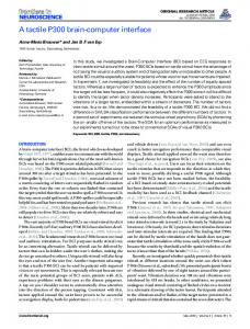
Fig. 3. Grand averaged ERPs of target stimuli across subjects 1-10 over 14 sites. Zero point is the beginning point of the target flash. The fringe of the shadow in each figure is the standard deviation of the ERP amplitude.
The number of trials per average was automatically selected based on the classifier output. After each trial, the classifier would determine the target character based on data from all trials in the specific trial-block. If the classifier chose the same item after two successive trials, the trial-block was terminated and the selected item was presented to the subject as feedback. For example, if the classifier selected “A” after the first trial, a second trial was presented. The data from both trials was averaged, and if the classifier selected “A” a second time no additional trials would be presented. If the classifier did not select “A”, another trial would begin, and so on until cha (n) = cha (n-1) or until 16 trials were presented.
After 16 trials, the classifier would automatically select the item with the highest classifier output [28]. 2.6. Subjective report After completing the last run, each subject was asked two questions about each of the two conditions. These questions could be answered on a 1-5 scale indicating strong disagreement, moderate disagreement, neutrality, moderate agreement, or strong agreement. The two questions were: (i) Were you attracted to the background at the target location? (ii) Did you perceive a distinct change in the shape of the matrix each time a flash occurred?
Instructions for Typing Manuscripts (Paper’s Title)
5
The questions were asked in Mandarin Chinese.
Fig. 4. Amplitude box-plots for each subject at four electrode locations (P8, Oz, Pz, and Cz). Amplitude is averaged from the maximum peak value ±25 ms for each electrode location. For each subject, the plot on the left represents the value for the SC-Pattern, and the plot on the right represents values for the MSC-Pattern.
Author’s Names
6
Fig. 5. Comparison of the topographic maps and time energy of r-squared values for SC-P and MSC-P; y coordinate is channel and x coordinate is time (ms).
3. Results Fig. 3 shows the grand averaged amplitude of target stimuli for all subjects and all 14 electrode locations used for classification. Fig. 3 clearly shows notable differences between the SC- and MSC-patterns. Averaged across all subjects, amplitude and latency values for the components of interest (i.e., N200, P300 and N400) are shown in table 1. Mean amplitude of the averaged ERPs (±25 ms) were compared between the two patterns using paired samples t-tests (see fig. 4). Electrode locations P8 and Oz were selected for the N200 analysis because MMN is typically largest in occipital areas [47, 49, 50, 56]. Electrode location Pz was selected for the P300 analysis because is commonly largest at Pz [17]. Electrode location Cz was selected for the N400 analysis because it typically contains the largest N400 [57]. Given that the N200 was compared at two electrode locations, a Bonferoni-Holm correction was used (α = 0.025). At electrode P8, although 7 of 10 subjects
showed larger N200s for the MSC-pattern, a statistically significant difference was not observed (t=2.2, p>0.025, Fig. 4A). At electrode Oz, N200 amplitude of the MSCpattern was significantly higher than the SC-pattern (t=3.7, p