490
IEEE TRANSACTIONS ON PARALLEL AND DISTRIBUTED SYSTEMS, VOL. 8, NO. 5, MAY 1997
A Parallel Algorithm for Graph Matching and Its MasPar Implementation Robert Allen, Luigi Cinque, Senior Member, IEEE, Steven Tanimoto, Fellow, IEEE, Linda Shapiro, Fellow, IEEE, and Dean Yasuda Abstract—Search of discrete spaces is important in combinatorial optimization. Such problems arise in artificial intelligence, computer vision, operations research, and other areas. For realistic problems, the search spaces to be processed are usually huge, necessitating long computation times, pruning heuristics, or massively parallel processing. We present an algorithm that reduces the computation time for graph matching by employing both branch-and-bound pruning of the search tree and massively-parallel search of the as-yet-unpruned portions of the space. Most research on parallel search has assumed that a multiple-instructionstream/multiple-data-stream (MIMD) parallel computer is available. Since massively parallel single-instruction-stream/multiple-datastream (SIMD) computers are much less expensive than MIMD systems with equal numbers of processors, the question arises as to whether SIMD systems can efficiently handle state-space search problems. We demonstrate that the answer is yes, and in particular, that graph matching has a natural and efficient implementation on SIMD machines. Index Terms—Graph, matching, parallel algorithm, SIMD, branch-and-bound, search, MasPar, combinatorial explosion, forward checking, load balancing.
—————————— ✦ ——————————
1 INTRODUCTION 1.1 Overview In many application areas, combinatorial search problems are common. These include computer vision, artificial intelligence, code optimization in compilers, and computeraided design. In practical situations, the sizes of the search spaces are so large that one often has to settle for solutions that are either suboptimal or based on more simplifying assumptions than would be ideal. In this paper, we give an algorithm that combines several techniques to speed up a particular optimization problem: the inexact matching of two graphs. The techniques we use include branch-andbound search, heuristics for computing good lower bounds on the distance between the two graphs, and massive parallelism. In addition, we formulate the algorithm to take advantage of single-instruction-stream/multiple-data-stream parallelism rather than the more flexible but much more expensive multiple-instruction-stream/multiple-data-stream sort of parallel system. This means that massively parallel processing can be more economically applied using our algorithm than would be the case with another algorithm.
————————————————
• R. Allen is with the Hewlett-Packard Company, Palo Alto, CA 94304. E-mail:
[email protected]. • L. Cinque is with the Dipartimento di Scienze dell’Informazione, Università “La Sapienza” di Roma, Via Salaria 113, 00198 Roma, Italy. E-mail:
[email protected]. • S. Tanimoto and L. Shapiro are with the Department of Computer Science and Engineering, Box 352350, University of Washington, Seattle, WA 98195. E-mail: {tanimoto, shapiro}@cs.washington.edu. • D. Yasuda is with the College of Ocean and Fishery Sciences, University of Washington, Seattle, WA 98195. E-mail:
[email protected]. Manuscript received 1 Aug. 1994. For information on obtaining reprints of this article, please send e-mail to:
[email protected], and reference IEEECS Log Number D95231.
Although we did address the issue of load balancing to some extent, the importance of our contribution lies in the formulation of our search and pruning methods to the massively parallel SIMD environment, and the integration of these three techniques to speed up graph matching. In the following paragraphs, we describe the application area that motivated our study: a problem in computer vision.
1.2 Motivating Application Model-based image analysis consists of constructing a structural description of a portion of an image, and then comparing this description to a model from a database of possible models. The determination of the probable identity of the objects in the image from the database of models involves two levels of search. The outer level is the search through the database to select those models that are most likely to match the structures extracted from the image. Then, finding the best such model requires an inner-level search, which is the process of evaluating how closely a model corresponds to the extracted structures. Most of the parallel approaches to model-based recognition in the literature (see Section 2) find the most likely model through a process of constraint satisfaction. These techniques have successfully reduced the cost of finding the best model; however, they are problem-specific rather than general techniques. Relational matching is a general approach to modelbased recognition that has been used by a number of researchers in the computer vision field [1], [2], [37], [38], [39], [40], [41], [42], [43]. Relational matching is a particular process for comparing structures which are represented as relational models. A relational model consists of a set of primitive parts and a description of the relationships among them. Two relational models are equivalent when a
1045-9219/97/$10.00 © 1997 IEEE
ALLEN ET AL.: A PARALLEL ALGORITHM FOR GRAPH MATCHING AND ITS MASPAR IMPLEMENTATION
bijection exists between the pieces of the first model and the pieces of the second that preserves all the relationships. Two relational models are similar if there is a one-one mapping from the pieces of the first model onto the pieces of the second that preserves most of the relationships. Similarity can be measured using the “relational distance” between two relational models [2]. When the relationships are binary, this reduces to the problem of finding a mapping between the vertex sets of two graphs that minimizes the value of a distance measure. Although our relational matching algorithm was motivated by applications in computer vision, it is not limited to this domain. It is a fully general graph matching algorithm limited neither to particular types of graphs, to particular applications, nor to particular types of computers.
1.3 Problem Formulation In this paper, we focus on the efficient solution of the graph matching problem in a parallel computing environment. The goal of the matching process is to find the best match between two graphs: G1, which we sometimes call the unit graph, and G2, which we sometimes call the label graph. (This terminology was introduced in [1].) We assume in our work that G1 and G2 have the same number of vertices. The best match can be considered as a permutation of the vertices of G1 so that as few of the permuted graph’s edges as possible differ from those of G2. For each possible permutation, the edges of G1 and G2 are compared, and an error of one is recorded for each unmatched edge. An unmatched edge can be an edge of G1 with no corresponding edge in G2 or an edge in G2 with no corresponding edge in G1. A simple example graph-matching problem is shown in Fig. 1. In this example we seek a permutation of the set {0, 1, 2, 3} of vertices of G1 that best aligns G1 with G2. In
Fig. 1. Two graphs, G1 and G2, to be matched.
Fig. 2. The search tree for permutations of {0, 1, 2, 3}.
491
this case there are three best permutations, each of which has an error of one. In the case of the permutation [0, 1, 3, 2] this is because the edge (3, 1) Œ G1 does not have a matching edge in G2; similar mismatches occur for the other two permutations. In Fig. 2, the tree of possible permutations and partial permutations for this problem is shown. Each branch of the tree represents the assignment of an element of the set to another (possibly the same) element of the set. At the first level, the element 0 is assigned either to itself, to 1, to 2, or to 3. At the second level, the possible assignments for element 1 triple the number of possible alternatives. At the third level, the number of possible alternatives doubles, whereas at the fourth level, the assignments for element 3 are fixed by the assignments of elements 0, 1, and 2. There are a total of 4! = 24 possible joint assignments (permutations) and each corresponds with one leaf node of the tree. The number of possible vertex permutations can be very large, growing as the factorial of the number of vertices of the unit graph. The number of possible mappings for a 15 vertex graph-matching problem is 360,360 times the number of mappings for a 10 vertex problem; the increased number of processors on a parallel machine can be quickly overcome by the problem size. Without clever means of finding cutoffs quickly, this number grows so rapidly that any standard backtracking scheme will take too long to be useful. One technique for pruning the search space is the use of a heuristic estimate of the cost of matching the unmatched portions of the graphs. This technique is called “forward checking” and we have described it in a previous paper [3]. The forward checking method employs a structure called the forward checking matrix (FCM) in its pruning algorithm. The rows of this matrix are indexed by unmatched
492
IEEE TRANSACTIONS ON PARALLEL AND DISTRIBUTED SYSTEMS, VOL. 8, NO. 5, MAY 1997
vertices in G1 and the columns by unmatched vertices in G2; its elements hold the independent error caused by mapping a presently unmatched vertex of G2. The main contribution of this paper is to present a new parallel algorithm for determining a minimum-distance correspondence between two graphs. In doing this, the algorithm finds the relational distance between two graphs. The paper is organized as follows. In the next section, we discuss the related literature in constraint satisfaction, object recognition, and parallel object recognition. In Section 3, we give a formal definition of our distance metric. In Section 4, we describe the SIMD parallel computing environment, the search algorithm, and how we manage the search process on the processor array. In Section 5, we present the results of our experiments on a 1,024 processor MasPar as well as on a DecStation serial processor. Section 6 contains the conclusions from our work. Detailed parallel pseudocode is included as an appendix.
2 RELATED WORK Graph matching plays an important role in various applications, such as computer vision, and the problem is closely related to constraint satisfaction, consistent labeling, and relaxation labeling. Solution approaches include “hierarchical synthesis” [4], in which one first looks for subgraph matches and then tries to extend them to larger mappings, and “inexact matching” [2], in which a distance measure called the relational distance between graphs is defined and used to determine the best mapping between two graphs. Constraint satisfaction has been studied extensively in computer vision and artificial intelligence [5], [6], [7], [8], [9], [10], [11], [12]. However, the object recognition comunity has done a great deal of work on matching that goes further than traditional constraint satisfaction does. For example, Bolles and Horaud [13] detected subgraph isomorphisms by finding maximal cliques in an association graph, and Umeyama [14] developed a polynomial-time method based on the eigendecomposition of the adjacency matrix of a graph; this technique obtains good results when the graphs are close to each other. The graph matching problem has also been attacked with strategies based on the generation and evaluation of hypotheses [15], [16], [17], [18]. Parallel methods have been studied for graph matching and other combinatorial optimization problems in both the computer vision and artificial intelligence communities, as well as in the computing community more generally. For example, parallel object recognition based upon tree search has been done on a Connection Machine CM-1 [19]. Geometric hashing can speed up graph matching for 3D vision problems [20]. Parallel hypothesis generation and testing for object recognition was demonstrated in [21], and other parallel object recognition methods are given in [22], [23], [24]. More general work on parallel search includes parallelizing the processing of individual nodes in the tree [25], tree decomposition [26], [27], [28], parallelizing alpha-beta search [29], and “parallel window search” [30]. An overview can be found in [31].
Combinatorial search on SIMD parallel architectures is problematical in part because search spaces are often irregular either in shape or in the relative importance of their subspaces, and also in part because the manipulation of graph structures typically involves manipulation of pointers or other symbolic representations. Consequently, it would seem necessary for the processors of a parallel machine to have autonomy at the level of SPMD architectures (single program/multiple data streams). Several authors have shown that SIMD systems are indeed capable of doing data-parallel combinatorial search. Iterative deepening search for solutions to the well-known 15-puzzle on an SIMD system was studied [32], [33], where the primary focus was on load balancing. A more theoretical study of the load balancing problem for SIMD combinatorial search can be found in [34], in which optimal conditions are derived for triggering load-balancing phases of the computation; they also test their method using the 15-puzzle on a Connection Machine CM-2 computer. The branch-and-bound method for combinatorial search is attractive whenever the objective function being minimized lends itself to easy computation of (relatively high) lower bounds. Computing distances between graphs fits nicely into this framework, as we will show later. One way to take advantage of parallelism for branch-and-bound search is to give different bounds to different processors in such a way that one processor is guaranteed to eventually find a solution, but other processors are made likely to find a solution quickly [35]. We note that parallel methods for branch-and-bound search can benefit from parallelization on massively-parallel computers in two other ways. First, processors can divide up the search space and process it more quickly together. Second, whenever one processor succeeds in improving the lower bound on the objective function, it can share it with all the others and thus enable them all to prune off more of their own subspaces from the search.
3 APPROACH 3.1 Basic Definitions Let G1 = ·V1, E1Ò and G2 = ·V2, E2Ò be two directed graphs to be matched. We assume for now that V1 = V2 = {0, 1, º, N - 1}. The sets of edges E1 and E2 are therefore both subsets of V1 ¥ V1, although we will often speak of E2 as a subset of V2 ¥ V2. We use both V1 and V2 in our presentation in order to make it clear which graph’s vertices we are referring to. We define the degree of mismatch d of a permutation p as the number of edges in G1 that are not mapped by p to edges in G2 plus the number of edges in G2 not mapped to edges in G1. d(G1, G2, p) = | E2 - {(p(vi), p(vj)) | (vi, vj) Œ E1} | + -1
-1
| E1 - {(p (vi), p (vj)) | (vi, vj) Œ E2} | The distance between two graphs is defined as the minimum d that can be obtained for any permutation p of the vertices. The problem of finding a permutation of one graph’s vertices to achieve a minimum distance from another graph
ALLEN ET AL.: A PARALLEL ALGORITHM FOR GRAPH MATCHING AND ITS MASPAR IMPLEMENTATION
is combinatorial in nature, and can be solved by a bruteforce backtracking tree search. Each iteration of the search answers the following question: Are there any unexplored paths from the root to a leaf going through the current node that might have a degree of mismatch less than the best value found so far? If there is such a path, the search process will move down the tree by adding an assignment for one more vertex to the partial permutation that corresponds to the next node along the path from the root to the current node, and then the question is asked again, etc. If there is no such unexplored path, the search moves back towards the root by removing the most recently added construct of the permutation. The path from the root to the current node in the search tree defines a partial permutation. A partial permutation pm
4 9
m m maps a subset V1 of V1 to a subset p m V2 of V2. The
members of
V1m
and
V2m
are said to be assigned under pm,
and the other vertices in V1 and V2 are said to be unassigned under pm.
3.2 Bound on the Degree of Mismatch Given a partial permutation pm, the search process needs to find a good lower bound for the degree of mismatch of all complete permutations containing pm, so that the search can be pruned as soon as possible. In order to provide a method for finding this lower bound, we need to examine the possible sources of mismatches. A mismatching edge of G1 in G2 according to pm can be classified into one of three groups: 1) an edge between a pair of nodes in G1 that have assigned image nodes in G2 under pm, 2) an edge between a node assigned an image node by pm and a node not assigned an image node by pm, and 3) an edge between two nodes not assigned image nodes by pm. In keeping with the terminology in our previous paper, the number of mismatching edges of the first type is called the past-past error, the number of the second type the past-future error, and the number of the third type the future-future error. Since the past-past error involves only the vertices of the graphs G1 and G2 whose correspondences are specified by pm, it can always be computed exactly by comparing the edges of the graphs. The past-future error is the error resulting from comparing those edges with exactly one incim dent vertex in V1 with corresponding edges in G2. The error resulting from these potential assignments can be placed into a data structure called the forward checking matrix (FCM). The FCM has one row for each unassigned vertex of G1 and one column for each unassigned vertex of G2. The entry FCM[i, j] represents the accumulated error for the mapping of the ith vertex of V1 to the jth vertex of V2. In practice, we maintain the FCM as an n ¥ n array, even though as a permutation is built up, the numbers of unassigned vertices in V1 and V2 get smaller and smaller. Each time we add another vertex assignment to the partial permutation, we simply ignore one more row and one more column of the n ¥ n array.
493
2
At the beginning of the search, the n coefficients of the FCM are initialized to zero, meaning that each potential vertex assignment has no error associated with it as yet. The values in the FCM are updated by the forward checking procedure, which is called every time a vertex assignment is added or removed from the partial permutation. The value of FCM[i, j] is incremented for each unmatchable edge in either G1 or G2 resulting from the addition of an assignment i ° j to the permutation being constructed. An example of an unmatchable edge would be an edge (vi, vk) in E1, for which no unmatched vertex l Œ V2 can be found for which ( j , l) is a corresponding edge in E2. By estimating a lower bound for the minimum error permutation in this matrix we estimate the lower bound for the error of any complete permutation containing pm. We call this estimation process “solving the FCM”; it is equivalent to solving a weighted bipartite matching problem. The future-future error is the number of mismatched edges between unassigned vertices. The future-future error constitutes a major portion of the potential distance between the graphs when the partial permutation is small and pruning is most effective. It cannot be exactly computed, because neither vertex incident to an edge is fixed; however, some information from the future-future error can be added to the forward checking matrix. If there are differences in the in-degree or out-degree between a vertex of G1 and a vertex of G2, then at least one edge mismatch must occur when these vertices are paired in the permutation. Although the estimated future-future error is often far smaller than the actual error that results from a full permutation, combining it with the FCM allows much earlier cutoffs than when using the past-past and past-future errors only. For future-future edges, using a simple counting mechanism can provide further information about error that would accumulate below a node were its descendants actually to be explored. For example, suppose there are 12 edges between four unmapped G2 vertices. These edges are counted at their source and sink vertices, providing an in-degree and outdegree for each unmapped vertex. These counts are expressed as (in-degree, out-degree) pairs for each G2 vertex, e.g., (7, 2), (3, 9), (2, 0), and (0, 1). Suppose the unmapped G1 vertices have (in-degree, out-degree) pairs of (3, 5), (6, 0), (1, 2), and (0, 3). Performing speculative mappings between G1 vertices and G2 vertices reveals edge deficiencies using either in-degree or out-degree. A table of all possible mappings for the vertices above gives the following deficiency information: IN-DEGREE
G1 vertices a b c d
OUT-DEGREE
G2 vertices A 4 1 6 7
B 0 3 2 3
C 1 4 1 2
D 3 6 1 0
G1 vertices a b c d
G2 vertices A 3 2 0 1
B 4 9 7 6
C 5 0 2 3
D 4 1 1 2
(In this example, we have V1 = {a, b, c, d} and V2 = {A, B, C, D}, departing from our earlier assumption that V1 = V2 = {0, 1, º, N - 1}. This makes it clearer where each element comes
494
IEEE TRANSACTIONS ON PARALLEL AND DISTRIBUTED SYSTEMS, VOL. 8, NO. 5, MAY 1997
from. The techniques involved are fundamentally the same.) Choosing the minimum path through the tables yields errors of two and six, respectively. Since any mapping must involve both the sources and sinks of edges, the greater of these can be used as a minimum bound. The errors from both of the tables cannot be combined at full value, since the tables reflect the same edge twice: once at its source vertex and again at its sink vertex. However, the tables may be combined after first multiplying them by scalars whose sum is 1.0, producing a result that is not greater than choosing the higher cost table. This is an advantageous approach because the cost of separately calculating errors for in-edges and out-edges to see which provides the better result is prohibitive. In this linear combination, both types of edges can contribute to the error calculation. The useful information from both the past-future and future-future errors is stored in tables with G2 vertices indexing the columns and G1 vertices indexing the rows. They are combined into a dense combined error matrix (CEM) before the more intensive work of finding a minimum path is performed. The CEM is used to determine the lower bounds on error for each child of a node. Since the children of a node correspond to the next G1 vertex being matched to each available G2 vertex in turn, a minimum bound for the combined future error for each child can be calculated as the minimum path through the CEM if the top row (the next G1 vertex) is matched to each column (each child). For instance, if the following is the CEM: G1 vertices a b c d
A 3 2 0 1
G2 vertices B C 4 5 9 0 7 2 6 3
D 4 1 1 2
then the four children of the current node would correspond to G2 vertices “A,” “B,” “C,” and “D” each being mapped to G1 vertex “a.” To calculate the future error of child (A, a), we take the error of three from the child’s place in the table and add the minimum path value (allowing a row to be chosen by only one column) through the remaining rows and columns. This path would be (B, d) (C, b) (D, c), resulting in an error of seven; the total minimum error for the (A, a) mapping is 10. The other children would have errors of six, 12, and 10, respectively. We call this process “solving” the matrix. This lower bound on future error can then be added to the past error of the current node to determine if it is possible for the child mapping to have an error under the current threshold. If not, the child can be eliminated. To solve the CEM by finding the minimum path requires its own combinatorial search. Shapiro and Haralick [1] gave a method to estimate the solution by choosing for each row the column with minimum value without breaking ties where two rows pick the same column. In a previous paper [3], we described two improvements on this algorithm. The first improvement was to calculate the higher error that must be incurred when more than one G2 vertex chose the same G1 vertex. The G2 vertex with the greatest difference
between its first and second choices would keep the contested G1 vertex, and the other G2 vertices would select their next-best choices. This second choice might result in further conflicts which were left unresolved; leaving the conflicts unresolved results in a lower error being projected from the matrix than would be the case if the minimum path were found. We found that the number of conflicts grew with the size of the CEM; one G1 vertex might be preferred by all the G2 vertices. This tendency resulted in a value far below that of the minimum path. Since the CEM is largest at the top of the tree (when the number of unmapped vertices is greatest), the technique is weakest when the potential savings from pruning is greatest. The second improvement was to reduce these conflicts by making the rows that are not chosen more competitive. This is done by calculating a value to subtract from each row; we found the most effective value for medium to large sized tables to be the fourth largest value in the row. This results in a leveling of the values in the matrix. The number of G1 vertices selected by some G2 vertex is increased, so that the resulting prospective mapping more closely resembles a minimum path. After the error of the prospective mapping is calculated, the sum of the values subtracted from the rows is added back.
4 THE PARALLEL ALGORITHM We implemented the parallel graph-matching algorithm on a MasPar MP-1 machine. In the following section, we describe the MasPar environment and explain the parallel algorithm in detail.
4.1 The MasPar Environment The MasPar MP-1 is a single instruction multiple data (SIMD) parallel processing computer consisting of an array control unit (ACU) and a relatively coarse-grained grid of processing elements (PEs) also referred to as “processors.” Our machine has 1,024 PEs, as compared to the 256,000 1-bit PEs on the Connection Machine CM-2. Each four-bit-wide processor has 32 32-bit registers on-chip and 64KB of offchip RAM. The ACU memory is termed “singular” and is readily accessible to any PE, while the memory on the PEs is termed “plural.” The PEs are arranged in a 32 ¥ 32 grid (array), indexed according to their position. Communication between PEs is accomplished either 1) neighbor-to-neighbor: Each PE can address the memory of its eight neighbors using the “X-net” interconnection scheme, 2) randomly via a global router, or 3) via the ACU: The ACU may poll from the array and broadcast to the array. Performing a branch-and-bound search with multiple instruction, multiple data (MIMD) machines has been shown to be no less efficient, in the sense of number of nodes expanded, than on a serial processor [36]. An SIMD processor is substantially less flexible; the speed-up for a search (in the sense of real time) compared to a serial machine is a fraction of the number of processors working on the search. However, the lower cost and the appropriateness of the SIMD system for lower-level image processing
ALLEN ET AL.: A PARALLEL ALGORITHM FOR GRAPH MATCHING AND ITS MASPAR IMPLEMENTATION
would likely make this architecture readily available for the higher-level tasks as well. A discussion of the changes to our algorithm that were required when it was moved from serial hardware to the MasPar is given following the explanation of the algorithm.
4.2 Summary of the Parallel Algorithm Much of the parallel algorithm for the MasPar involves identical logic to that of a serial algorithm; we implemented a serial version of the algorithm for comparison in our experiments. The algorithm presented below has the form of a sandwich: Steps unique to the parallel environment occur on either side of steps that a serial search would perform. 1) Initialize processor array: Read in data, partition search space among processors—each processor may get several branches (jobs) loaded into its job queue. 2) LOOP until all subproblems on each of the processors have been treated (the subspaces completely searched or eliminated by pruning). a) All processors with work to do perform the following branch-and-bound search loop in parallel for the lessor of a constant number of iterations or until the branch is fully explored: i. selection of subproblem ii. expansion of subproblem iii. termination test and update of the local incumbent (best permutation and corresponding degree of mismatch) iv. elimination test b) Scan all processors for new global incumbent. c) Scan all processors to determine if all nodes are explored. d) Inactive processors read in new jobs from their job queues. e) Perform load balancing if the number of inactive processors with empty queues is above a threshold. 3) Output the final incumbent and the relational distance found.
4.3 Initializing the Processor Array As implied by its classification, an SIMD implementation must have multiple data streams for the single instruction stream to manipulate. In our data-parallel approach, the first task of parallelization is to partition the search space among the processors. In order to explain the partitioning algorithm, we first describe the search tree. To represent all possible mappings of G1 vertices to G2 vertices, we employ a search tree in which each horizontal level represents a G1 vertex and each node of that level represents a potential G2 vertex to correspond to it (but at the second and deeper levels, there generally are multiple nodes for each possible G2 vertex). The root of the tree will have N branches, since the first G1 vertex may be mapped to any of the G2 vertices. Each of these branches will have N - 1 branches, since a G2 vertex cannot be simultaneously mapped to more than one G1 vertex. Continuing this process down N levels results in N! leaf nodes or possible mappings, and each root-to-leaf path is a unique permutation of the G2 vertices. Therefore, the set of all paths from root to leaf in an N vertex mapping problem is equivalent to the set of all per-
495
mutations of the integers from zero to N - 1, a fact we use to maintain the distinction between neighboring subproblems that may be present on widely separated processors. Using permutations, we have developed a means of representing the needed partitions of the search space in a highly efficient manner. A subtree (a subproblem) can be completely designated by a pair ·H, bÒ, where H is the permutation representing the path from the root to the subproblem’s left-most leaf, and b is defined as the depth of the root of the subtree that represents the subproblem. For example, in a subproblem ·[2, 0, 1, 3, 4], 2Ò, there are six of the 120 possible permutations; the first of the six is [2, 0, 1, 3, 4] and the last of them is [2, 0, 4, 3, 1]. The portion of the permutation from the root to a subtree root is fixed for a subproblem. The branches from the subtree root are the set of all permutations of the G2 vertices not used in the fixed portion. Each node of the tree will have as many branches (children) as the distance between it and the bottom level (this distance is N - b). (Equivalently, the number of G2 vertices still available is the distance to the leaf, and any of the available G2 vertices can be mapped to the next G1 vertex.) This is recursively true as we move down the tree: The G2 vertices that make up any path from a node to a descendant leaf are identical to the children of the node. Each processor is initialized with a queue of subproblems in the following way. We start by calculating how many subproblems are required to provide all processors with work. Each processor can have an active job and several jobs waiting in a queue. Let q be the number of entries allocated for each processor’s queue. Let n be the number of processors on the machine. Then nq is the total number of queue entries allocated on the machine. Partitioning the tree evenly by expanding all the branches at the top level will create N subproblems. Expanding the next level will result in N(N - 1) subproblems, and so on. Therefore it is simple to calculate Nb, the number of equal-sized subproblems we can easily generate that will fit into the nq job queue entries, and b, the number of levels of expansion required to produce those Nb subproblems. Since all the branches at a given level will be expanded, all subproblems are initially the same size. Note, however, that some fraction of the PEs are likely to have one more job in their queues than the others, since the number of subproblems is not likely to be a multiple of the number of processors. So the task is to partition the tree at level b, so that each processor has roughly the same amount of work to do. For an illustration of the job allocation process, take the number of processors to be six, the queue size to be five, and the number of vertices in the graphs to be mapped as five. The tree can be split at the second level to produce twenty jobs, and still fit within the 30 available queue entries. Using the terms above, n = 6, q = 5, N = 5, nq = 30, Nb = 20, and b = 2. The desired result of the allocation process is the following: PE0: ·[0, 1, 2, 3, 4], 2Ò, ·[0, 2, 1, 3, 4], 2Ò, ·[0, 3, 1, 2, 4], 2Ò, ·[0, 4, 1, 2, 3], 2Ò. PE1: ·[1, 0, 2, 3, 4], 2Ò, ·[1, 2, 0, 3, 4], 2Ò, ·[1, 3, 0, 2, 4], 2Ò, ·[1, 4 , 0 , 2 , 3], 2Ò.
496
IEEE TRANSACTIONS ON PARALLEL AND DISTRIBUTED SYSTEMS, VOL. 8, NO. 5, MAY 1997
PE2: PE3: PE4: PE5:
·[2, 0, 1, 3, 4], 2Ò, ·[2, 1, 0, 3, 4], 2Ò, ·[2, 3, 0, 1, 4], 2Ò. ·[2, 4, 0, 1, 3], 2Ò, ·[3, 0, 1, 2, 4], 2Ò, ·[3, 1, 0, 2, 4], 2Ò. ·[3, 2, 0, 1, 4], 2Ò, ·[3, 4, 0, 1, 2], 2Ò, ·[4, 0, 1, 2, 3], 2Ò. ·[4, 1, 0, 2, 3], 2Ò, ·[4, 2, 0, 1, 3], 2Ò, ·[4, 3, 0, 1, 2], 2Ò.
There are two approaches to achieving this initial job distribution: 1) make it the responsibility of the serial host computer, or 2) devise a parallel algorithm such that the SIMD machine can do it by itself. Since the latter is more interesting, we describe such a method below. Each processor will calculate the left-most permutation of the job that belongs in each of its queue entries. Each queue entry is initialized with the left-most permutation of the whole tree; in our example, this would be [0, 1, 2, 3, 4]. This permutation also represents the N children of the root of the search tree. We use both meanings of the permutation in our initialization process: At any iteration i, the first i slots of the permutation are fixed, describing a vertical path in the tree, while the remaining slots of the permutation describe the children of the ith node. The first iteration of our process is for each queue entry to calculate which branch of the root node it belongs to, establishing the element in the first slot of the permutation. The method of calculation will be explained below. The occupant of the first slot is swapped with the new first element; for example, if three was calculated, the initial permutation would be modified into [3|1, 2, 0, 4], which contains a mark showing what choices have been made so far (the elements to the left of the vertical bar). In the second iteration, each queue entry calculates which of the children of the first node it belongs to. The resulting element is again swapped with the occupant of the second slot; for example if two was calculated, the resulting marked permutation is [3, 2|1, 0, 4]. The calculation can be repeated again with the queue entries calculating which child belongs in its third slot, and so on. In our example, we need only assign the first two elements, so we are done after the second iteration. The final step establishes the left-most branch of the subtree by writing the unused elements into the remaining slots in ascending order. In the example, this would result in [3, 2, 0, 1, 4]. Each processor will calculate which elements it should select for its permutation using a unique number that is systematically modified as successive elements are assigned through the iterative process. Let xi represent this identifier at the ith iteration. The initial value x0 is made to be a unique identifier for each queue entry; x0 is obtained by adding the unique processor ID (with the first processor having an ID of 0) to the product of the number of processors times the position of the entry in the queue (with the first queue entry being at position 0). In the example, the third queue entry for the fifth processor would have an x0 value of 16, because x0 = 4 + (6 * 2). The selection of the first element is calculated for each queue entry by taking x0 modulo N. Any surplus queue spaces (those above Nb) are left empty. This results in Nb/N queue entries selecting each child of the root node. Our
example case would map element 1 to 1, since 16 modulo 5 equals 1, with the resulting marked permutation being [1|0, 2, 3, 4]. In our example system, four queue entries (those with x0 equal to 1, 6, 11, and 16) would assign themselves to the branch of the tree starting with one. The second element is chosen by first calculating x1 as the greatest integer less than or equal to x0/N. This partitions the queue entries so that the first N entries (which have each selected successive children from the root node) have x1 equal to 0, the next N entries have x1 equal to 1, and so on, with the last N entries having a value of N - 1 for their x1. The element belonging to the second slot of the permutation is calculated by taking x1 modulo N - 1. This calculation allows each queue entry to select which child of the first node it should map to the second G1 vertex. Since there are N - 1 branches from each level-one node, and by definition N - 1 is a factor of Nb, there will be one queue entry for each available child of the first level node. In our example case, x0 was 16, so x1 is 3, which indicates that this entry should take the element from the permutation with index 3, which is the element 4 (since our index starts with 0 at the current position). Now the example queue entry would be [1, 4|2, 3, 0]. Our small example is finished after the second iteration, since b = 2, so the cleanup step of assigning unused elements in ascending order is performed, with the resultant permutation being [1, 4, 0, 2, 3]. For actual problems, the algorithm can continue to map elements as necessary. The first step in deriving the (i + 1)th mapping is to take xi as the greatest integer less than or equal to x0 i- 15
0 5
N - i-1
The (i + 1)th element’s index is xi mod N - i. This cycle is repeated until level b of the tree is reached; each level-b node will be represented by one and only one queue entry in the processor array.
4.4 The Search In order to have the processors of the SIMD explore the search space in parallel, we have developed a simple algorithm that a processor can use to generate all leaf nodes (permutations) in a subproblem. The process is to inspect the vector describing the current permutation H from right to left, comparing each element of the permutation to its left neighbor. Let the ith element of the permutation H be designated by H[i]. Let H[i] be the element on the left, so H[i + 1] is the element on the right. If H[i] has a lower value than H[i + 1], then swapping the two will create a new permutation corresponding to a path in the search tree that is to the right of the path corresponding to H. If no such path is found while i ≥ b, then this subproblem is complete and there are no branches to the right to be expanded. While finding that H[i] < H[i + 1] indicates a branch exists to the right of that for the value H[i], the branch for H[i + 1] may not be the next one in the ordering of the tree. Therefore, it is necessary to inspect the tail of the permutation (elements H[i + 1] through H[N]) to find the element closest to and greater than H[i], which indicates the next branch to the right. Since the next branch
ALLEN ET AL.: A PARALLEL ALGORITHM FOR GRAPH MATCHING AND ITS MASPAR IMPLEMENTATION
to the right should have only branches to the left below the i level, we precede with this inspection with sorting the tail of H into ascending order. Now it is simple to inspect the tail of the permutation starting at H[i + 1] from left to right until the first element exceeding H[i] is found and exchanged with H[i]. For example, with b = 2, N = 6, and a starting permutation of [0, 1, 2, 4, 5, 3], the successor permutation is [0, 1, 2, 5, 3, 4]. An initial mismatch threshold is input with the graphs to be matched. If a permutation, or all possible permutations below a given node, can be determined to have a degree of mismatch above the threshold, the node and its descendants can be eliminated from further consideration. If a complete permutation is found which has a degree of mismatch below the threshold, its degree of mismatch becomes the new threshold, and the permutation is stored as the new incumbent (best permutation known so far to this processor). The processors are scanned for improvements in the lowest degree of mismatch found, and a global best permutation and new threshold are established. This process continues until all permutations have been checked or pruned away. The branch-and-bound search process consists of four components: 1) 2) 3) 4)
selection of subproblems, expansion of subproblems, termination testing and updating of the incumbent, and elimination tests.
The search is performed through iterating these steps. The selection of the next subproblem is done through a simple ordering of nodes; each processor investigates a subproblem from left to right, without evaluating which branch may have the best chance for providing a minimal degree of mismatch. Therefore, the process of selection of the next subproblem is blind; if a branch is not eliminated by the elimination tests, it is expanded. Suppose a processor is at a node in the “middle” of its subproblem; that is, the node is at a level c such that b < c < N - 1. The basic search process performed by each processing element is an iteration of a loop that either expands a child node (moving down the tree), expands the next node on the same level (moving up to the parent and back down to a sibling to the right), or closes a node (moving up the tree to the parent). The first two options require determining whether the node expanded provides a complete permutation (the “termination test”). If it does not provide a complete permutation, the algorithm must evaluate whether any children of the node should be eliminated (the “elimination test”). If a complete permutation is available, the relational distance associated with this permutation is checked against the threshold, and the local incumbent permutation is updated as appropriate. When moving up the tree, the level reached is compared against b, the depth of the subproblem root, to determine whether the subproblem has been completed. The heart of the elimination process is to evaluate the children of the current node to determine whether further work needs to be done. The three types of error are com-
497
bined for children of the current node to determine whether any can be eliminated from further consideration: 1) error from edges between mapped vertices (past-past error), 2) error from edges between a mapped vertex and an unmapped vertex (past-future error), and 3) error from edges between unmapped vertices (futurefuture error). Each processor has its own FCM which has columns corresponding to G2 vertices and rows corresponding to G1 vertices. Due to the restricted amount of memory available to each processor, we do not retain separate FCMs for each tree node or each level of the search. Instead, each processor updates a single table of its own as it moves through its subproblem’s search tree; a traversal of a single arc in the tree generally affects only a small portion of the FCM. Therefore, the process is one of updating the table— modifying it when we move down the tree and updating it in reverse when moving back up the tree. All of the branch-and-bound functions described above can be performed in parallel, since each processor’s subtree can be processed in isolation from other parts of the search tree. Besides having more processors doing the work, the chief benefit from the parallel approach is having quick updating of all processors with a new threshold as soon as it is found. After a constant number of cycles (we have found 200 is acceptable for large graphs), the processors that have finished their jobs can extract a fresh job from their queues, reinitialize their tables, and continue the search process. Once a processor has completed the work in its queue, it remains idle until the next load-balancing cycle arrives.
4.5 Load Balancing The mechanism we developed for load balancing has two phases. The first phase is for the processors with jobs remaining in their queues to move them to processors that are idle. The second phase is performed when, after this redistribution of jobs, a significant number of processors (we found this level to be best set at about 20%) still have no work to do. In this case, the processors that have jobs split them into equal parts, one for each unexpanded child of the job’s root node. This new multiplicity of jobs may overfill the processor’s job queue, in which case the final job will be all the remaining children. Next, the queue-sharing cycle is repeated, spreading jobs throughout the processing array. Our original plan was to split the tree as much as necessary to keep the processors constantly active. However, we were surprised by the additional work created by splitting the tree. The processors were far more active, but they had far more work to do, and the overall time was lengthened. To evenly spread the work from processors that have untouched jobs in their queue to those with no work at all, we have each processor look to its neighbor to the east. This is done toroidally, that is, the eastern-most column of processors considers the western-most column of the processor array as its neighbor. If the neighbor of a processor has more work than the original processor, it moves a job to
498
IEEE TRANSACTIONS ON PARALLEL AND DISTRIBUTED SYSTEMS, VOL. 8, NO. 5, MAY 1997
its own queue. This process is repeated c times, where c is the number of columns in the processor array. This sharing is then repeated with each processor looking to its neighbor to the south r times, with r equal to the rows of the processor array. These two cycles insure that no processor will have more than one more job in its queue than any other. As mentioned above, a job can be completely designated by the pair ·H, bÒ, where H is defined as the permutation representing the path from the root to the job’s leftmost leaf, and b is defined as the depth of the node which is the root of the subtree which represents the subproblem. To split the job, b is incremented, and a new permutation H is defined for each child of the original branch-node. If the job being split is the active job, new permutations H are only created for the children to the left of the child involved in the current search. Since this process is creating copies of H, the fixed portion of the tree is being replicated for each child. The number of copies and the amount of fixed tree being copied are inverses, and the number of fixed nodes added is greatest at the point half way from the root to the leaf. When a job is loaded from the queue, it is initialized at the root of the tree; it must perform a move down the tree along the fixed path until it reaches b. These added moves, when multiplied over all the processors splitting jobs, quickly outweighed the benefit of always having all the processors active. We have found superior performance when we allow up to 20% of the processors to become idle before splitting up jobs.
4.6 Parallel Implementation Considerations The following are the main limitations of the MasPar hardware and their effects on our algorithm. 1) SIMD Execution: Because the ACU sequentially broadcasts instructions to the processor array, branches and loops that are dependent on plural data will cause some processors to be idle while others are active; consequently, more statements will be executed from the code than on a serial machine (e.g., all the statements in an “if º else” structure will be executed). One of the challenges in designing an SIMD algorithm is to minimize these situations in the code, maximizing the number of active processors. One technique is to add a small number of initializing statements to manipulate the plural data, aligning the processors and eliminating the need for separate branches to handle the different situations. 2) Four-Bit Processing Elements: Because of the small size of the processor, plural data is stored as eight-bit characters whenever possible. Because of the multiple cycles required for each step and the lower-level technology, we found program execution time to be about 27 times longer on a single PE operating as a serial processor than on a DecStation 5000 serial machine. This hardware performance level reduced the real-time theoretical hardware advantage of the MasPar from a ratio of 1,024:1 to something closer to 40:1. The processing time for real number arithmetic is substantially longer than integer arithmetic; however, our algorithm does not use any real variables.
3) Off-Chip PE Memory: Memory access speeds were found to vary greatly. Let Tr denote the time required for a PE to access an on-chip register. PE access to offchip RAM is 4Tr. PE access to RAM using an indirect lookup with a RAM pointer is 8Tr. This constraint can be ameliorated in some situations by explicitly naming register variables in code where one would normally use a “for” loop and an array with an incrementing index. When arrays are necessary, they should be as dense as possible to minimize lookups. It is also possible to overlap the RAM access time with calculations by making an assignment to a register from an array several instructions before the value will be used. 4) Inter-PE Communication: The time required for neighbor-to-neighbor communication is very little more than local RAM access time (4Tr), and posed no constraint. Communication between PEs using the Router without conflicting destinations takes about 85Tr and was not used in our algorithm (conflicting destinations can slow the process tremendously). We found that a PE could receive a value broadcast from the ACU in time Tr/2, faster than from any other source, probably because it is using the same path that instructions use. For the ACU to scan the array (a reduction operation) for a minimum (or maximum) value takes approximately 50Tr. These reduction operations are necessary to detect new thresholds for pruning the search tree, and their value quickly outweighs their cost, especially in the initial phases of the search.
5 EXPERIMENTS AND RESULTS The results of our experiments with graph matching are presented in two areas: the number of search tree nodes expanded (or the number of “moves”), and the real time required to complete a given search. The number of moves required to solve a given problem is highly data-dependent and anomalies are common [36]. For instance, if the vertices of the graph have homogenous characteristics and the best mapping has a relational distance close to the error of many mappings, fewer cut-offs will be found and the search will take longer than for a graph with sharp differentiations. Moves are counted when expanding a branch, moving across the tree to a sibling, as well as when moving up the tree. Therefore, the number of moves is higher than the number of search tree nodes expanded; the figure is intended to be used as a comparison with the serial algorithm. Our experiments were performed using the test graphs listed in Fig. 3. We implemented a serial version of our algorithm on a DecStation 5000 and tested several of the mappings on both it and the 1,024 processor MasPar. For the larger graphs the time required on the serial machine became prohibitive; the table shows n/r for no results in these cases. The number of parallel moves are expressed in three ways: The first column shows the number of move cycles performed by the algorithm; the second shows the number of potential nodes explored in that number of cycles (Column 1 * Number of
ALLEN ET AL.: A PARALLEL ALGORITHM FOR GRAPH MATCHING AND ITS MASPAR IMPLEMENTATION
Reference
Number of Vertices
Number of Edges
Average Edges/ Vertex
Number of Possible Mappings
m10a
10
25
2.5
3.629 ¥ 10
m10d
10
40
4.0
3.629 ¥ 10
m13a
13
25
1.9
6.227 ¥ 10
m13b
13
30
2.3
6.227 ¥ 10
m15a
15
20
1.3
1.308 ¥ 10
m16a
16
20
1.25
2.092 ¥ 10
m17a
17
25
1.4
3.557 ¥ 10
m18a
18
25
1.4
6.402 ¥ 10
m27l
27
64
2.4
1.089 ¥ 10
m27u
27
64
2.4
1.089 ¥ 10
graph with those of the other. The algorithm achieves speed through a combination of features: branch-and-bound search, good bound estimation through the use of the forward-checking matrix, efficient generation of permutations by the processors of the SIMD system, and massive parallelism. Furthermore, by formulating the algorithm to run on the SIMD class of parallel machine, we are able to take advantage of the economies that such machines offer over MIMD systems. It might be possible to improve our algorithm further by
6 6 9 9
12 13
1) making the bound-computation heuristics even better through deeper lookahead in the forward-checking matrix, 2) incorporating the more sophisticated load-balancing methodology of Karypis and Kumar [34] where additional testing of a triggering condition is done in order to balance the load precisely when it becomes too unbalanced.
14 15 28 28
Fig. 3. Characteristics of test graphs. Graphs Matched m13a
m13b
m16a m16a
DEC 5000 Moves
Cycles
MasPar Potential
Moves
3,249
94
97,008
64,604
m15a
57,795
494
509,808
311,526
m16b
107,123
434
447,888
248,480
m17a
m18a
2,304,475
4,495
m27l
m27u
n/r
300,511
4,638,840 3.75 * 10
9
3,749,637 3.65 * 10
9
Fig. 4. Comparison of search moves on MasPar and DecStation. Graphs Matched m13a m13b m16a m15a m16a m16b m17a m18a m27l m27u
DEC 5000 Time 6 sec. 103 sec. 205 sec. 70 min. n/r
499
MasPar Time 8 sec. 54 sec. 46 sec. 9.7 min. 25 hours
Fig. 5. Actual time required to complete searches.
Processors); and the third shows the actual number of moves made on the tree by all processors (Column 2 - Idle Processor Cycles). Fig. 4 shows the results in terms of moves for several graphs. When graphs of different sizes are compared, the smaller graph is enlarged with “dummy” vertices without edges, so the problem size is always the size of the larger graph. The real times taken for the problems in Fig. 4 are shown in Fig. 5. These results show that the increased overhead and slower processing rates make the MasPar a liability for smaller problems. It is only in searches involving more than 16 vertices that the MasPar consistently outperforms the DecStation in real time terms. However, once that line is passed, the performance of the serial processor falls far behind the MasPar.
6 CONCLUSIONS We have presented an algorithm for finding the relational distance between two graphs. It searches the space of all permutations of the N vertices of one graph to find a best correspondence between the nodes (and edges) of one
Both of these enhancements, however, incur additional overhead, and only additional experimentation will be able to determine whether they bring savings in practical situations.
7 APPENDIX ALGORITHM DESCRIPTION IN PSEUDOCODE Pseudocode for Next Leaf Generation from Permutation function NextPerm(array H[0 .. N - 1, int b) i := N - 2; while ë (i ≥ b) do if ë(H[i] < H[i + 1]) then begin there is a branch to the right at the i level, but we need to find the next larger node, which may not be in H[i+1] at this time j := i + 1; SortArrayAscending(H[j]..H[N - 1]) whileí( j £ N - 1) do if ë (H[i] < H[j]then ë Swap(H[i], H[j]); j := N - 1; endif j := j + 1; endwhile i := b; end endif i := i - 1; endwhile
terminates loop
terminates loop
For example, with b = 4, N = 6, and the start branch = [0, 1, 2, 4, 5, 3], the result branch = [0, 1, 2, 5, 3, 4].
ACKNOWLEDGMENTS This research was supported in part by U.S. National Science Foundation Grants Number IRI-9023977 and CDA9123308, by NASA/CESDIS, and by the Boeing Company.
500
IEEE TRANSACTIONS ON PARALLEL AND DISTRIBUTED SYSTEMS, VOL. 8, NO. 5, MAY 1997
REFERENCES [1] [2] [3] [4] [5] [6] [7] [8] [9] [10] [11] [12] [13] [14] [15]
[16]
[17] [18] [19] [20] [21] [22] [23] [24] [25] [26] [27]
L.G. Shapiro and R.M. Haralick, “Structural Descriptions and Inexact Matching,” IEEE Trans. Pattern Analysis and Machine Intelligence, vol. 3, pp. 504–519, 1981. L.G. Shapiro and R.M. Haralick, “A Metric for Computing Relational Description,” IEEE Trans. Pattern Analysis and Machine Intelligence, vol. 7, pp. 90–94, 1985. D. Yasuda, L. Cinque, L.G. Shapiro, S. Tanimoto, and R. Allen, “An Improved Algorithm for Relational Distance Graph Matching,” Pattern Recognition, pp. 349–359, 1996. H.G. Barrow, A.P. Ambler, and R.M. Burstall, “Some Techniques for Recognizing Structures in Pictures,” Frontiers of Pattern Recognition, pp. 1–29, Academic Press, 1972. D.L. Waltz, “Understanding Line Drawing of Scenes with Shadows,” The Psycology of Computer Vision, Winston, ed., pp. 19–91, 1975. U. Montanari, “Networks of Constraints: Fundamental Properties and Application to Picture Processing,” Information Science, vol. 7, pp. 95–132, 1974. E.C. Freuder, “Synthesizing Constraint Expression,” Comm. ACM, vol. 21, no. 11, pp. 958–966, 1978. B.A. Nadel, “Constraint Satisfaction Algorithms,” Computational Intelligence, vol. 5, pp. 188–224, 1989. E.C. Freuder, “A Sufficient Condition of Backtrack-Free Search,” J. ACM, vol. 29, no. 1, pp. 24–32, 1982. R. Dechter and J. Pearl, “Network-Based Heuristics for Constraint-Sotisfaction Problems,” Artificial Intelligence, vol. 34, pp. 1–38, 1987. P.V. Hentenryck, Y. Deville, and C.-M. Teng, “A Generic ArcConsistency Algorithm and Its Specializations,” Artificial Intelligence, vol. 57, pp. 291–321, 1992. V. Kumar, “Algorithms for Constraint-Satisfaction Problem: A Survey,” AI Magazine, pp. 32–44, Spring 1992. R.C. Bolles and P. Haraud, “3DPO: A Three Dimensional Part Orientation System,” Int’l J. Robotics Research, vol. 5, no. 3, pp. 3–26, 1986. S. Umeyama, “An Eigendecomposition Approach to Weighted Graph Matching Problem,” IEEE Trans. Pattern Analysis and Machine Intelligence, vol. 10, no. 5, pp. 695–703, Sept. 1988. N.J. Ayache and O.D. Faugeras, “HYPER: A New Approach for the Recognition and Positioning of Two-Dimensional Objects,” IEEE Trans. Pattern Analysis and Machine Intelligence, vol. 8, no. 1, pp. 44–54, Jan. 1986. W. Eric, L. Grimson, and T. Lozano-Perez, “Localizing Overlapping Parts by Searching thr Interpretation Tree,” IEEE Trans. Pattern Analysis and Machine Intelligence, vol. 9, no. 4, pp. 469–482, Apr. 1987. A.K. Jain and R. Hoffman, “Evidence-Based Recognition of 3D Objects,” IEEE Trans. Pattern Analysis and Machine Intelligence, vol. 10, no. 6, pp. 783–802, June 1988. I. Gaudron, “2D Objects Recognition by Graph Matching,” Proc. ICPR, vol. II, conf. B, pp. 508–511, 1992. J.G. Harris and A.M. Flynn, “Object Recognition Using the Connection Machine’s Router,” Proc. Computer Vision and Pattern Recognition, pp. 134–139, 1986. I. Rigoutsos and R. Hummel, “Massively Parallel Model Matching—Geometric Hashing on the Connection Machine,” Computer, vol. 25, no. 2, pp. 33–42, Feb. 1992. L.W. Tucker, C.R. Feynman, and D.M. Fritzsche, “Object Recognition Using the Connection Machine,” Proc. IEEE-CVPR 88, pp. 871–878, 1988. T.A. Cass, “A Robust Parallel Implementation of 2D Model-Based Recognition,” Proc. IEEE-CVPR 88, pp. 879–884, 1988. T.S. Newman, A.K. Jain, and R.J. Enbody, “3D Object Recognition: Interpretation Tree Search on a MIMD Machine,” Proc. ICPR 92, vol. I, pp. 337–340, 1992. C.C. Reinhart and R. Nevatia, “Issues in Parallel Tree Search for Object Recognition,” Proc. ICPR 92, vol. IV, pp. 225–228, 1992. C. Ebeling, All The Right Moves. MIT Press, 1987. V.N. Rao, V. Kumar, and K. Ramesh, “A Parallel Implementation of Iterative-Deepening-A*,” Proc. AAAI 87, pp. 178–182, 1987. V.N. Rao and V. Kumar, “Parallel Depth-First Search, Part I: Implementation,” Int’l J. Parallel Programming, vol. 16, no. 6, pp. 479– 499, 1987.
[28] V. Kumar and V.N. Rao, “Parallel Depth-First Search, Part II: Analysis,” Int’l J. Parallel Programming, vol. 16, no. 6, pp. 501–519, 1987. [29] R. Feldmann, B. Monier, P. Mysliwietz, and O. Vornberger, “Distributed Games Tree Search,” Parallel Algorithms for Machine Intelligence and Vision. Springer-Verlag, 1989. [30] G. Baudet, “The Design and Analysis of Algorithms for Asynchronous Multiprocessors,” PhD dissertation, Computer Science Dept., Carnegie-Mellon Univ., 1978. [31] V. Kumar, P.S. Gopalakrishnan, and L.N. Kanal, Parallel Algorithms for Machine Intelligence and Vision. Springer-Verlag, 1990. [32] A. Mahanti and C.J. Daniels, “A SIMD Approach to Parallel Heuristic Search,” Artificial Intelligence, vol. 60, pp. 243-282, 1993. [33] C. Powley, C. Ferguson, and R.E. Korf, “Depth-First Heuristic Search on a SIMD Machine,” Artificial Intelligence, vol. 60, pp. 199241, 1993. [34] G. Karypis and V. Kumar, “Unstructured Tree Search on SIMD Parallel Computers,” IEEE Trans. Parallel and Distributed Systems, vol. 5, pp. 1,057-1,072, 1994. [35] V. Kumar and L.N. Kanal, “Parallel Branch-and-Bound Formulations for AND/OR Tree Search,” IEEE Trans. Pattern Analysis and Machine Intelligence, vol. 6, pp. 768–778, 1984. [36] B.W. Wah, G.J. Li, and C.F. Yu, “Multiprocessing of Combinatorial Search Problems,” Computer, vol. 18, no. 6, pp. 93–108, June 1985. [37] J.K. Cheng and T.S. Huang, “Image Registration by Matching Relational Structures,” Pattern Recognition, vol. 17, no. 1, pp. 149– 159, 1984. [38] B. Radig, “Image Sequence Analysis Using Relational Structures,” Pattern Recognition, vol. 17, no. 1, pp. 161–167, 1984. [39] A. Wong and M. You, “Entropy and Distance of Random Graphs with Application to Structural Pattern Recognition,” IEEE Trans. Pattern Analysis and Machine Intelligence, vol. 7, no. 5, pp. 599–609, May 1985. [40] K.L. Boyer and A.C. Kak, “Structural Stereopsis for 3D Vision,” IEEE Trans. Pattern Analysis and Machine Intelligence, vol. 10, no. 2, pp. 144–166, Feb. 1988. [41] B. Yang, W.E. Snyder, and G.L. Bilbro, “Matching Oversegmented 3D Images to Models Using Associated Graphs,” Image and Vision Computing, vol. 7, no. 2, pp. 135–143, 1989. [42] G. Vosselman, Relational Matching. Berlin: Springer-Verlag, 1992. [43] K. Sengupta and K.L. Boyer, “Information Theoretic Clustering of Large Structural Modelbases,” Proc. IEEE Conf. Computer Vision and Pattern Recognition, pp. 174–179, 1993. Robert Allen received the MS degree in computer science from Stanford University in 1995. His studies focused on distributed systems, machine learning, and databases. He is currently a software engineer at the Hewlett-Packard Company’s Palo Alto site. His interests include object-oriented languages and the research and development of information systems to support design and manufacturing.
ALLEN ET AL.: A PARALLEL ALGORITHM FOR GRAPH MATCHING AND ITS MASPAR IMPLEMENTATION
Luigi Cinque (S’85, M’90, SM’96) received his PhD degree in physics (and computer science) from the University of Napoli in 1983. After a few years at the Artificial Intelligence Laboratory (Selenia S.p.A.), where he worked on artificial intelligence, expert systems, and knowledgebased vision systems, in 1990, he joined the Department of Computer Science at the University “La Sapienze” of Rome, as an assistant professor. There he works on object recognition, parallel architectures, and algorithms for image processing and computer vision. In 1992, he was a visiting scientist at the University of Washington (Seattle) working on parallel machines. His current interests include computer vision, parallel image processing and architectures, pattern recognition, 3D object recognition, and spatial database systems. Dr. Cinque is a senior member of the IEEE, and a member of the ACM, the Pattern Recognition Society, and the American Association of Artificial Intelligence. He is an editorial board member of Pattern Recognition. Steven L. Tanimoto received the AB from Harvard in 1971 and the PhD from Princeton in 1975. He is currently a professor of computer science and adjunct professor of electrical engineering at the University of Washington in Seattle. His research interests include visual languages, educational technology, parallel image processing, and artificial intelligence. He has held visiting positions at the University of Paris, Linköping University (Sweden), Kobe University (Japan), the National Institutes of Standards and Technology, and Thinking Machines Corporation. Dr. Tanimoto served as an associate editor of IEEE Transactions on Pattern Analysis and Machine Intelligence from 1983 to 1986, and as editor-in-chief from 1986 to 1990. His text, The Elements of Artificial Intelligence Using Common Lisp, second edition, was published by W.H. Freeman in 1995. He served as the program chair for the 1992 International Workshop on Visual Languages, the 1994 International Conference on Pattern Recognition subconference on parallel computation, and as co-program chair of the 1994 IEEE Computer Society Conference on Computer Vision and Pattern Recognition. He is a fellow of the IEEE.
501
Linda G. Shapiro received the BS degree in mathematics from the University of Illinois, Urbana, in 1970, and the MS and PhD degrees in computer science from the University of Iowa, Iowa City, in 1972 and 1974, respectively. She was an assistant professor of computer science at Kansas State University, Manhattan, from 1974 to 1978, and an assistant professor of computer science from 1979 to 1981 and associate professor of computer science from 1981 to 1984 at Virginia Polytechnic Institute and State University, Blacksburg. She was director of intelligent systems at Machine Vision International in Ann Arbor, Michigan, from 1984 to 1986. She is currently a professor of computer science and engineering and of electrical engineering at the University of Washington, Seattle. Her research interests include computer vision, image database systems, artificial intelligence, pattern recognition, and robotics. She has coauthored two textbooks, one on data structures and one on computer and robot vision. Dr. Shapiro is a fellow of the IEEE and a member of the Pattern Recognition Society and the American Association for Artificial Intelligence. She is a past chair of the IEEE Computer Society Technical Committee on Pattern Analysis and Machine Intelligence and is currently an editorial board member of IEEE Transactions on Pattern Analysis and Machine Recognition and Pattern Recognition. She has served as editor of CVGIP: Image Understanding, co-program chair of the IEEE Conference on Computer Vision and Pattern Recognition in 1994, general chair of the IEEE Workshop on Directions in Automated CAD-Based Vision in 1991, and general chair of the IEEE Conference on Computer Vision and Pattern Recognition in 1986. She has also served on the program committees of numerous vision and AI workshops and conferences. Dean Yasuda received an MA degree in mathematics from the University of San Diego in 1990. He is a research analyst and software developer for the University of Washington’s Columbia Basin Research, a project devoted to the study and preservation of the Pacific Northwest wild salmon runs.


![Graph theory and its applications [Book Review] - IEEE ... - IEEE Xplore](https://m.moam.info/img/260x300/graph-theory-and-its-applications-book-review-ieee_5baa4e93097c47566d8b4752.jpg)