A Parallel Implementation of the Cylindrical Algebraic ... - CiteSeerX

A Parallel Implementation of the Cylindrical Algebraic Decomposition Algorithm B. David Saunders Hong R. Lee Department of Computer & Information Sciences University of Delaware Newark, Delaware 19711 S. Kamal Abdali y Division of Computer & Computation Research National Science Foundation Washington, DC 20550

Abstract

ti er elimination. Here the given formula may contain free variables, and the problem is to nd a quanti erfree formula logically equivalent to the given one. For example, (8x)[x2 + bx + c  0] contains free variables b and c, and a logically equivalent quanti er-free formula is b2 ? 4c  0. If the given formula has no free variables, then the result of eliminating quanti ers is a formula which is just TRUE or FALSE. The rst algorithm for quanti er elimination was given by Tarski [17] in 1940. Although important theoretically for establishing that the theory of real closed elds is decidable, this algorithm turns out to be too inecient to be of any practical use. The cylindrical algebraic decomposition (CAD) algorithm was invented by Collins [9] in 1973. A full implementation of the CAD algorithm was completed in 1981 by Arnon in the computer algebra system SAC2. A variant of the algorithm using clustering was later implemented in SAC2 also [3]. The CAD algorithm has found use in several areas other than quanti er elimination, e.g. robot motion planning [15], term-rewriting systems [10], algebraic topology [12], and computer graphics [1]. Algorithms other than Collins' have been proposed, e.g. [6, 7, 13, 14] and important improvements in the CAD approach have been oered, e.g. [5]. But at present no other algorithms have been implemented, and no complete implementation of even the CAD algorithm is available in any computer algebra system other than SAC2. The CAD algorithm is doubly exponential in the number of real variables involved, and, in practice, can only solve rather small problems in a reasonable time. Nonetheless, many interesting and, indeed, unsolved problems can be expressed by a reasonably sized state-

In this paper, we describe a parallelization scheme for Collins' cylindrical algebraic decomposition algorithm for quanti er elimination in the theory of real closed elds. We rst discuss a parallel implementation of the computer algebra system SAC2 in which a complete sequential implementation of Collins' algorithm already exists. We report some initial results on the speedup obtained, drawing on a suite of examples previously given by Arnon.

1 Introduction The elementary theory of Algebra and Geometry or theory of real closed elds is in essence the matter of deciding the validity of statements which can contain quanti ers and logical connectives and in which the atomic formulae consist of polynomial equations and inequalities. For example, (9x)(8y)[(x2 + y2 > 1)&(xy  1)] is such a statement. The more general problem is that of quan This work has been supported by the National Science Foundation under Grant No. CDA-8805353. y The statements contributed by this author to this paper represent his personal opinions, and should not be construed as the ocial viewpoint of the National Science Foundation.

1

2 Parallelizing SAC2

ment in the theory, involving only a few variables. This pilot project explores the potential to increase the universe of solvable problems in the theory by exploiting multiprocessing.

The CAD algorithm, implemented by Collins and his students, was written in ALDES and depends on his extensive library, SAC2, of algebraic procedures. The rst step in this eort was to adapt the SAC2 library for parallel execution on multiple processors. They are written in ALDES, which is translated into FORTRAN. The FORTRAN versions are then compiled and archived appropriately on a given machine and le system. At run time the routines call each other in various patterns, including recursive calls. Parameters and other variables manipulated for the most part are list structures representing algebraic entities. To handle the situation, variables are of type integer from FORTRAN's point of view. They serve as pointers to list cells. In SAC2 this means they are indices for the global shared array SPACE. The other fundamental data structure of the system is the STACK array. The STACK, for each routine in the library, holds variables which must be subject to garbage collection. In SAC2 parlance, these variables are \unsafe". The SPACE array holds the list cells which are the basic units of all the data manipulated by procedures in the system. The basic need to adapt to the multiprocessor environment is to arrange for a stack for each process, while maintaining a common SPACE in shared memory. The stack for each process could be a private local entity, but we chose to make the STACK a global common entity like SPACE. For multiprocessing it is partitioned into segments, one for each process. If the STACK array has n elements unused at the time of multiprocess forking, and the machine has p processors, then each processor operates with its stack being a segment of length n=p in the global STACK array. There are two reasons for this choice. For one, a side eect of the scheme is that any process can access any other processor's stack. This capability is used in some versions of garbage collection with which we have been experimenting. Secondly, if each processor is to have a private local stack, there must be an eective way to share that stack with subroutines. A subroutine must share P 's stack when called by P and Q's stack when called by Q. We didn't feel we had an appropriate (relatively machine independent) mechanism in the FORTRAN available to us on the Sequent to handle this situation. An additional consideration in the stack implementation is the handling of the current stack pointer, INDEX. In the parallel version there must be an INDEX for each processor. We handle this by creating an array PINDX of p stack pointers, one for each process. Subroutines in the library call IUP when they start. This updates the INDEX appropriately. We replace this with PIUP, which uses the processor id to access and update the appropriate entry in PINDX and also set a local variable INDEX. Then the references to INDEX in the remainder of the

Parallel processing architectures can provide dramatic speedup in the time needed to perform many computations, including algebraic ones. Here we obtain a speedup by using coarse grained parallelism on a multiprocessor with tens of processors and shared memory. Examples of such machines are the Sequent Balance and Symmetry models, the Encore Multimax, and the BBN Butter y. The computations reported here were performed on a Sequent Symmetry with 8 processors. In contrast to MIMD machines and the coarse grained approach taken here, one might consider SIMD designs and ne grained parallelism. Such an approach works best on homogeneously structured data, so that the synchronous processing can be eective. However, most data in algebraic computation is highly heterogeneous. For example, consider matrices whose entries are polynomials in several variables of diering degrees and term lengths. Computations on such matrices will call for subcomputations on the entries which dier dramatically in detail of instruction sequence and in time required. This makes it dicult to obtain good speedup on SIMD machines, with important exceptions for speci c problems (see for example Johnson [11]). On the other hand, with appropriate dynamic scheduling of tasks and load balancing good speedup may be obtainable using coarse grained parallelism on MIMD designs. In our experiments the processors operate asynchronously and communicate through shared memory. The risk exists that communication costs may override the bene ts of the multiprocessing. However we have experienced approximately 50% eciency in this initial eort (see Section 5 for details). From this modest experience we oer the modest conjecture that a factor of 10 speedup can be obtained on a wide range of computer algebra computations from a 20 processor machine. The rest of the paper is organized as follows: Section 2 outlines the changes made to the SAC2 library to support parallel computation. Section 3 gives a brief overview of the CAD algorithm with references to the literature, and Section 4 describes the modi cations made to the algorithm in order to parallelize the most time consuming portion, the extension phase. Section 5 oers the results of some timing experiments and preliminary analysis of the data. Finally, some conclusions and observations on these experiments are drawn in Section 6. 2

Problem No. Description 1 Ellipse, 1 Mw space, 4 GCs 2 Ellipse, 2 Mw space, 2 GCs 3 Ellipse, 4 Mw space, 1 GC 4 Quartic, 2 Mw space, 0 GCs 5 Quartic, 0.2 Mw space, 2 GCs 6 SIAM, 2 Mw space, 0 GCs 7 SIAM, 0.1 Mw space, 1 GCs 8 Pair-5, 2 Mw space, 1 GC1 9 Tacnode, 2 Mw space, 11 GC 10 Implicit, 2 Mw space, 70 GC 11 Pair2, 2 Mw space,

Time Total GC Net Total GC Net Total GC Net Total

1 316.01 18.73 297.28 314.92 18.08 296.84 415.71 47.61 368.10 40.63

2 196.33 17.08 179.25 201.26 16.57 184.69 352.35 82.65 269.70 33.72

No. 3 153.81 12.59 141.22 158.20 12.00 146.20 336.54 103.33 233.21 30.04

Total GC Net Total

42.69 1.77 40.92 14.69

29.72 1.62 28.10 14.68

25.68 1.15 24.53 12.95

of processors 4 5 132.20 118.83 9.93 8.63 122.27 110.20 137.72 124.01 9.35 8.03 128.37 115.98 267.05 255.46 63.35 64.66 203.70 190.81 28.11 26.98 23.75 0.88 22.87 12.63

Total 15.01 9.50 7.77 6.95 GC 0.45 0.40 0.29 0.23 Net 14.56 9.10 7.48 6.72 Total 250.76 150.70 126.93 98.06 GC 8.52 7.82 5.47 4.12 Net 242.24 142.88 121.46 93.94 Total 1607.06 897.58 865.15 847.00 GC 94.50 86.36 60.62 45.77 Net 1512.56 811.22 804.53 801.23 Total 12976 7021 5110 4936 GC 629 553 405 322 Net 12346 6467 4704 4613 Total 34985 23657 13636 13335 # GCs (194) (196) (199) (199) GC 1751 1639 1125 864 Net 33234 22018 12511 12470 1 GC time counted from the rst PE arrival

22.46 0.75 21.71 12.10

6 109.59 7.66 101.93 114.46 7.07 107.39 259.62 72.94 186.68 25.98

7 105.26 7.30 97.96 110.47 6.71 103.76 263.73 66.68 197.05 25.76

21.59 0.65 20.94 10.97

21.07 0.61 20.46 11.74

6.83 6.13 6.13 0.19 0.16 0.15 6.64 5.97 5.98 96.08 94.69 95.39 3.48 3.03 2.85 92.60 91.66 92.54 842.81 835.44 837.01 38.66 33.37 31.53 804.15 802.07 805.48 4883 4810 4781 280 295 286 4603 4514 4494 13241 13141 13096 (199) (199) (199) 763 677 633 12478 12463 12462

Figure 1: Execution times for parallel extension and parallel GC

3

code are valid and the number of modi cations needed is kept to a minimum. Since a global SPACE array is constantly accessed and modi ed by all processes, there are, of course, some subroutines where greater adjustment is required to handle the mutual exclusion requirements and avoid racing conditions. In particular, routines which modify list structure (routines which write on SPACE) must be written carefully. Chief among these is COMP (the SAC2 equivalent of Lisp CONS). Mutual exclusion must be assured in the section in which COMP detaches a cell from the available cell list. Secondly, if no cells are available, garbage collection must be initiated, a process which aects the whole computation and involves all processors. At least, this is the case for SAC2's simple mark and sweep garbage collector where we make no attempt to do incremental or local garbage collection. Our approach to garbage collection depends on the assumption that all processes will access the available cell list often (usually through COMP). There is a barrier at the beginning of garbage collection. The assumption is that processors can aord to spin at this barrier because other processors will soon also need a new cell, discover there are none, and join the earlier arrived ones at the barrier. When all processors have arrived, garbage collection commences. Our rst implementation ignored one important situation in which this assumption (that all processes will seek new cells) is invalid. This situation occurs when, near the end of the parallel computation, some processes nd no work left to do (see the section below on the CAD implementation) and exit. It is not hard to see that such a process will indeed not seek new cells. Our solution to this is greedy. We have nished processors spin on a GC

ag. When an un nished processor discovers the need for garbage collection, it raises the ag, and nished processors join the active ones at the barrier and participate in garbage collection. Our data indicates that this solution works well (see Section 5). Garbage collection itself is done in two phases separated by a barrier. First each processor marks cells reachable from its STACK segment, then spins at a barrier until all processes are through marking. Next, each processor sweeps an assigned region in SPACE, and links the available cells it obtains into the global available cell list. The synchronization for the latter is managed by a lock. Parallel performance can be heavily dependent on communication costs. In our situation the most uncertain and dicult to analyze or predict are the eects of SPACE array accesses. Each processor has a local cache. A high proportion of cache hits among the memory accesses is very valuable. In addition, there can be considerable contention on the bus for some memory access patterns. The data below, though not extensive, fails to

show any serious problem in this area, at least for the CAD algorithm.

3 Cylindrical Algebraic Decomposition Below we give a very brief description of the CAD algorithm, referring the reader to [4] for a thorough discussion of the algorithm and to [2] for a comprehensive bibliography of CAD theory and applications and other related work. Let A be a nite set of polynomials in r variables with integer or rational coecients. Let E r denote the r-dimensional Euclidean space. The CAD algorithm decomposes E r into a nite set of cells (disjoint, connected sets), in which at every point each polynomial in A has the same sign. This decomposition has two important properties: 1. It is cylindrical in the following sense: Given a region (a nonempty connected subset) R of E k , the set R  E is called a cylinder (over R). The cells obtained in the decomposition of E r can be joined into cylinders over certain regions of E r?1 , which can, in turn, be joined into cylinders over certain regions of E r?2, and so on. 2. The decomposition is also algebraic in the sense that the cell boundaries are the zeros of certain polynomials obtained from the polynomials of A. The CAD algorithm works in three phases: 1. Projection. From the given polynomials in r variables, polynomial resultant and discriminant operations are used to construct new polynomials containing, successively, r ? 1, r ? 2, ... , 1 variable(s). The so obtained k-variate polynomials have the property that their zeros are projections of certain critical aspects of the (k + 1)-variate polynomials, such as intersections and tangents to the direction of projection. 2. Base. The real zeros of the univariate polynomials obtained in the last step of the projection phase are used to decompose E 1 into cells which are either points (corresponding to polynomial zeros) or open intervals (between the zeros). Since each polynomials in A has the same sign throughout each of these intervals, a convenient rational sample point is chosen for each interval. 3. Extension. From the base phase decomposition of E 1 , successive decompositions of E 2 , E 3 , ... , E r are derived. This is done by erecting cylinders over cells of lower dimensions, and partitioning 4

these cells into regions throughout which appropriate polynomials from the projection phase have the same sign. During the extension from E k to E k+1 , the (k + 1)-variate polynomials (obtained during projection) are evaluated at the sample points in the cells of E k , giving just univariate polynomials. The zeros of these polynomials provide the (k +1)st coordinates that, combined with the k coordinates of the cells over E k , determine the decomposition of E k+1 . The application of the CAD algorithm to the quanti er elimination problem is brie y as follows: Consider a logical formula which is comprised of logical connectives and quanti ers and in which the atomic formulae are equations and inequalities involving polynomials in r variables. The variables are assumed to range over real numbers. First consider the case in which the formula contains no free variables. In this decision problem what matters is the sign pattern| that is, the sequence of signs (positive, zero, or negative)| of the values of the polynomials (in some order) at all r-tuples of real numbers. The CAD algorithm decomposes the entire r-dimensional real space into a nite number of cells which are invariant as to sign pattern of the polynomials. Hence, one can determine whether the given formula is true or false from the values of the polynomials at the sample point of each cell. In the case that there are free variables in the formula, the algorithm uses the describing polynomials for each cell to construct a quanti er formula equivalent to the original formula. Problem Number 1 2 3 4 5 6 7 8 9 10 11

Execution Time Coecients a

b

Sequent provides a FORTRAN preprocessor based on parallelizing DO loops with the DOACROSS directive [16], essentially a stripmining technique. This is of no use to us, since SAC2 is completely devoid of DO loops. Sequent also provides a suite of multitasking primitives, centered around a routine, mfork, which forks a speci ed number of identical processes. We used this suite for our parallelization. Other somewhat more machine independent approaches are possible, but Sequent's multitasking system was quite suitable for this pilot project. The extension phase of the CAD algorithm was chosen for parallelization for two reasons. First, it dominates the time of computation in most instances. Second, it consists of completely independent work building a cylinder over each cell. The clustering versions of CAD do not have such complete independence, and clustering was not attempted here. However, we do not think that clustering is a signi cant impediment to parallelization. The sequential CAD algorithm does the extension phase in a loop controlled by a structured list S of cells. Each loop iteration takes one cell and produces in its place the list of cells one dimension higher in the cylinder over the original cell. We use dynamic scheduling to parallelize this loop. First a copy S0 of the structured list, with entries all zero, is created. Then a subroutine is mforked to run on p processors. The subroutine on each processor repeats the following 1. Take one cell from S (under lock), 2. extend the cell, creating a list s of higher dimension cells, and 3. Replace by s the zero in S0 in the position corresponding to the cell initially taken from S. Note that this does not have to be synchronized in any way.

Fit & Error Coecients c

u

v

77 241 -1 2.4 .008 87 230 -2 3.6 .01 297 133 -10 43.7 .10 27 14 -1 .9 .02 17 26 0 .2 .005 15 1 -1 1.2 .08 4 11 0 0.3 .02 40 208 3 11.0 .04 176 1333 73 120.5 .07 -453 12897 509 405.2 .03 3479 31494 682 4041.1 .12

When no cells remain in S, processors spin at a barrier until all are done. Then a single processor replaces S by S0 and makes a copy as before in preparation for extension to the next dimension. The process is repeated r ? 1 times as we extend from 1 dimension to r dimesions. When no dimensions remain, nished processors spin on a GC ag as mentioned in the discussion of GC in Section 2. The cell lists could very naturally be implemented as a shared database, in the style of the Linda [8] parallel programming system.

Figure 2: Timing model for parallel execution

5 Timing Data and their Interpretation

4 Parallelizing Cylindrical Algebraic Decomposition

We ran the sequential as well as the parallel version of the CAD algorithm on a number of problems taken from Arnon [3]. The problems attempted are the following:

We now describe how we have modi ed the CAD algorithm to run it on the Sequent Symmetry computer. 5

Time

seq.

23.13 46.93 47.66 3 259.44 4 GC time 14 94 271.99 5 Speedup Eciency ? 257.05 5 ? 23.80 2 1 211.78 4? 3 w/o GC 196 84 235.58 p Speedup Eciency T1 T2 T T

:

T

T

GC

T

T

T

T

:

T

1 26.5 53.90 54.66 301.20 18 08 314.59 .84 .84 296.51 27.04 246.54 228 46 273.58 .86 .86 :

:

2 26.66 48.38 49.16 188.16 16 57 201.55 1.34 .67 184.98 21.72 139.00 122 43 160.72 1.47 .73 :

:

No. of processors(parallel) 3 4 5 6 7 26.26 26.38 26.21 26.35 26.33 44.24 40.94 41.48 40.79 39.36 45.02 41.72 42.26 41.56 40.14 145.63 122.14 110.69 101.76 96.22 11 99 9 34 8 01 7 05 6 69 159.05 135.55 124.12 115.19 109.66 1.71 2.00 2.19 2.36 2.48 .57 .50 .44 .39 .35 147.06 126.21 116.11 108.14 102.97 17.98 14.56 15.27 14.44 13.03 100.61 80.42 68.43 60.20 56.08 88 62 71 08 60 42 53 15 49 39 118.59 94.98 83.70 74.64 69.11 1.99 2.48 2.81 3.16 3.41 .67 .62 .56 .53 .49 :

:

:

:

:

:

:

:

:

:

Figure 3: Timing of program segments

 Pair-5. The input polynomials for CAD are 27xy + 9x2 ? 31x + 4; 5y3 ? 14xy2 + 15y2 + 13x2y + 2xy + 14y ? 7x3 ? 3x:  Tacnode. The input polynomial for CAD is y4 ? 2y3 + y2 ? 3x2 y + 2x4 :

 Ellipse. This example originates in the problem to

determine whether the ellipse de ned by the equation (x ? c)2 + (y ? d)2 = 1 a2 b2

lies (without touching) wholly inside the circle de ned by x2 + y2 = 1. Actually, at present the CAD implementations have only succeeded in solving the special case when d = 0. The input formula for quanti er elimination is therefore

 Implicit The input polynomials for CAD are 505t3 ? 864t2 + 570T + x ? 343; 211t3 ? 276t2 ? 90t ? y + 345:  Pair-2 The input polynomials for CAD are 9y2 + 30xy ? 22x2 + 21; 2y3 ? 12x2 y ? 12xy ? 8y + 11x2 ? 2x ? 2:

(8x)(8y)((ab 6= 0 & b2 (x ? c)2 + a2 y2 ? a2 b2 = 0)

) x2 + y2 ? 1  0) The input presented to the CAD algorithm for the timings below consists of the following polynomials obtained by some manual projection and simpli cation [3]:

a; a ? 1; b; b ? 1; b ? a; c; c ? 1; c +1; c + a +1; c + a ? 1;

We ran the parallel version of the CAD program by varying the number of processors from 1 through 7. Although our Sequent Symmetry con guration has eight processors, there is a system constraint that only seven processors can be taken over for exclusive use of an application program. For the Ellipse problem, we also varied the size of the SPACE array of SAC2 from 1 to 4 Megawords (Mw). When garbage collection occured in any run, we recorded the garbage collection time also. For these runs, we thus have both the total CPU time and the net time not including garbage collections. The results are shown in Figure 1 where the times are given in seconds.

c ? a + 1; c ? a ? 1; b2c2 + b4 ? a2 b2 ? b2 + a2 :

 Quartic. The input polynomials for CAD are p; 8pr ? 9q2 ? 2p3; 256r3 ? 128p2r2 + 144pq2r + 16p4 r ? 27q4 ? 4p3 q2 :  SIAM. The input polynomials for CAD are 144y2 + 96x2y + 9x4 + 105x2 + 70x ? 98; xy2 + 6xy + x3 + 9x: 6

Problem No. Description 1 Ellipse

2 Tacnode

Time Expansion Idle times

total Expansion Idle times

total

No. of processors 1 2 3 4 5 247.26 143.10 104.19 80.31 68.37 0 1.47 1.20 1.62 .85 0 .43 .33 .65 0 .25 .46 0 .04 0 0 1.47 1.63 1601.49 891.93 859.52 0 3.23 576.41 0 7.28 0

0

2.20 841.42 827.22 821.35 4.51 0

2.0 837.20 825.93 823.61 820.00 3.82 0

6 61.56 1.53 1.44 .87 .58 .23 0 4.65 829.15 819.81 819.63 815.75 813.77 3.24 0

3.23 583.68 1653.08 2473.36 3272.20

7 56.70 1.73 1.30 .90 .79 .37 .27 0 5.36 831.41 823.65 822.70 821.90 817.71 816.35 4.36 0 4106.67

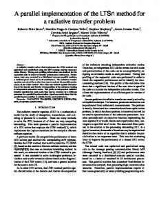
Figure 4: Processor idling after exit from extension phase Except where indicated, the GC times are measured from the time the rst processor detects the need for GC. We also have measured the time the last processor encounters lack of available list cells, and arrives at GC. The resulting times are insigni cantly lower, indicating that the approach taken to parallel GC works ne in this context. In the Ellipse problem, we note that as the SPACE array is increased from 1 to 2, then to 4 Mw, the number of garbage collections decreases from 4 to 2, then to 1. The net CPU time in signi cantly higher for the 4 Mw SPACE array. Since this means that the memory demand of the program is above the 16 Mb physical memory, the penalty is probably due to increased memory swapping to disk. The improvement when we go from 2 Mw to 1 Mw is less pronounced and we conjecture that it is accounted for by the hardware design. Each processor has a 64 kb cache. Memory access time is fastest when (the valid instance of) the data addressed is in one's own cache, slower if it is in another processor's cache, and still slower when it is in main memory. When the SPACE array is smaller, a greater portion tends to reside in the caches. To further test the increased performance with smaller SPACE, We tried smaller sizes. The Ellipse problem runs out space when the size is much below 1 Mw. However, Figure 1 shows that the bene t of smaller space is even more pronounced when the size 0.1 Mw is used for the problems Quartic and SIAM. To analyze the timing data obtained in our experiments, we looked for a t to the following model. Suppose there are p processors working in parallel. Then the time for executing a task should be a function of the

form

a + pb + cp;

where a, b and c are constants that depend on the task. Here, a represents the part of the task that cannot be distributed among the processors, while b represents the parts that can be simultaneously performed by parallel processors. Even if the third term is deleted from the above formula, a non-zero value of a means that the speed up in performing the task is not perfectly ecient. But, in fact, matters are worse because there are parts in most tasks for which adding more processors can actually increase the exceution time. The purpose of the coecient c is to account for such parts. For example, some processor initialization has to be done sequentially, once for each processor. More seriously, since in a shared-memory machine such as the Sequent, all processor/memory communication takes place over a common bus, increasing the number of processors creates bottlenecks in the bus, and increases processing time. In the above model, we assume that such overheads are just proportional to the number of processors used, ignoring any quadratic or higher-order eects. Figure 2 shows the values of a, b, and c that have been derived using a least-squares t over the data in Figure 1. The values u, and v provide a measure of the absolute and relative accuracy of the t. Speci cally, the derivation of the quantities in Figure 2 is done as follows: Let A be the 7  3 matrix whose i th row is the vector [1; 1=i; i]. Then x = [a; b; c]T is the best least squares t to a solution of Ax = k, where k is the vector of the last seven numbers in each row of Figure 1. 7

Furthermore, u is the 2-norm of (Ax ? k), the absolute error of the best solution, and v is u=(2-norm of k). Note that according to the above formula, the larger the value of b is compared to a and c for a program, the closer the program comes to achieving ecient linear speedup. Below we compare one of these ts with detailed measurements of parallel and sequential segments of the computation. Just from the overall timings given in Figure 1, one can draw some conclusions about this model. It has some validity when the t is extremely good, v < :01 say. But in problem 8 (Pair-5), for example, the coecients suggest a successful parallelism; b = 208 is substantially larger than a = 40 and c is negligible. However, Figure 1 shows that the performance is essentially uninproved after p = 4, probably due to the computation time of two or three individual cell extensions. We then recorded timings for individual sections of the computation to reveal the extent to which the model suggested above describes the sequential and parallel portions of the computation. In the table below, T1 through T5 denote clock readings at various points of the computation. The clock reading at the beginning is zero. 1. T1 is the elapsed time to the beginning of extension. this rst phase is on a single processor. 2. T2 is the end of univariate extension into E 2 , which is done in parallel.

One may compare the time spent in the nonparallelized sections of the program, approximately 40 seconds, with the value a = 101 from the previous table. This shows that 60% of the \sequential" time from the model T = a + b=p + cp is due to costs of synchronization and memory contention in the parallel phase. Indeed, as calculated, the eciency of the speedup is around 40% and degrading slightly as p increases. We believe substantial improvements can be made in these gures by arranging that more of the computation be in local memory instead of the almost complete dependence on the global SPACE array as done here. Because of the highly independent nature of the extension of each cell in the CAD algorithm this localization should be very successful. It is less clear how well it will work when one includes adjacency and clustering calculations, which also should be done. To further study the nature of eciency losses, we measured the variation in the idle time of the processors at the end of each extension phase. Extension involves the construction of cylinders over n cells, requiring times t1 ; :::; tn . The times may be quite variable and the mapping onto p processors may be far from ideal. At the worst, the dierence between the time the rst processor exits (for lack of more cells to extend) and the time the last processor exits is the maximum of t1 ; :::; tn . Figure 4 shows the idle times that occur as the processors exit the extension phase. The two problems shown reveal the extremes. For Ellipse the load is quite well balanced, whereas for Tacnode, there are two processors busy for the duration, and p ? 2 idle for most of the time. Thus for Tacnode, at the granularity we are exploiting, the bene ts of parallelism are limited by the two largest ti . To overcome this would require exploitation of parallelism at a ner granularity, namely in the individual cell extensions, i.e., in the real root isolation algorithm. Also note for Ellipse that since there is little idle time as the processors exit the extension phase, the eciency losses (around 50%) are due to costs spread throughout the extension computation. They are due to locking and unlocking, references based on a processor id variable and the like. Parallelism at a ner granularity will not help here. It will only add overhead costs. For this type of problem, subprocesses need greater independence and lower overhead. The challenge seems to be to achieve greater independence of the subprocesses (less dependence on the single shared SPACE) and adaptive granularity.

3. T3 is the end of a brief single processor stage to initialize the structured list of cells for bivariate extension. 4. T4 is the end of the second extension phase into E 3 , done in parallel. All garbage collection occurs during this extension. 5. T5 is the end of the computation, after a nal single processor phase. 6. Tp is (T2 ? T1) + (T4 ? T3 ), the total time spent in the parallel phase. 7. For T5 and Tp the speedups, (sequential time)/(pprocessor time), and the eciencies of the speedups, speedup/p, are also shown. The times for the parallel version of the program on one processor are about 16% greater than the times for the sequential algorithm. This applies to the uniprocessor sections as well as the (potential) multiprocessor sections of the parallel algorithm. We suspect that this may be explained almost entirely by the cost of the lock on AVAIL, the available space list, which is invoked at every use of COMP.

6 Conclusions We have implemented a parallel version of the SAC2 library, and have successfully parallelized the CAD algorithm. To our knowledge, this is the rst parallel im8

plementation of an important, very large computer algebra program. To many computer algebra professionals, SAC2 is a bit unattractive because of its FORTRAN base and primitive interface. But the FORTRAN code of SAC2 turned out to be a blessing in disguise for us, because FORTRAN ts quite naturally in the Sequent parallel programming environment. Of course, a Cbased computer algebra system, such as Maple, would also be relatively easy to parallelize. But as yet the CAD algorithm has not been written in any C-based system. To parallelize a Lisp-based system (e.g. REDUCE or Macsyma) would be rather dicult at present. Although there exist certain parallel versions of Lisp, the dierences in constructs between sequential and parallel Lisps would require one to essentially recode major parts of the system in order to parallelize it. When new procedures are written in ALDES, our approach requires some manual modi cation to the intermediate FORTRAN code. It would be desirable, and not terribly involved, to modify the ALDES translator to handle the needed variant forms for parallelism. At the present state of parallel programming tools and environments, the parallelization of a large program takes much eort. Required is a thorough analysis of the sequential code in order to determine parallelizable parts of algorithms, critical sections, variable classi cation with respect to their locality to processes and their dierent modes of access by processes, etc. Moreover, each new architecture and operating environment seems to require all this work to be redone. For this reason, we are quite intrigued by, and plan to experiment with, the Linda system [8] which promises to be an architectureindependent environment for writing parallel programs. Our implementation seems to have a 40{50% eciency (the ratio of speed-up to the number of processors used). Although we would certainly like to improve it, we feel that an order of magnitude speed-up is possible even with the current implementation on a fully con gured machine.

[2] [3] [4]

[5] [6] [7] [8]

[9]

[10] [11]

7 Acknowledgement

[12]

Ruth Shtokhamer initiated the project to parallelize SAC2. Dennis Arnon explained and clari ed several aspects of the CAD algorithm to us. He (with further improvements by Jeremy Johnson) is also the author of the QE-interface program which makes working with the CAD algorithm in nitely simpler than in the raw SAC2 version.

[13] [14] [15]

References [1] Arnon, D. S.: \Topologically reliable display of algebraic curves", Proc. ACM SIGGRAPH '83, De-

[16] 9

troit, MI, 219{227. (1983) Arnon, D. S.: \A bibliography of quanti er elimination for real closed elds", J. Symbolic Computation, 5, 267{274. (1988) Arnon, D. S.: \A cluster-based cylindrical algebraic decomposition algorithm", J. Symbolic Computation, 5, 189{212. (1988) Arnon, D. S., Collins, G. E., McCallum, S.: \Cylindrical algebraic decomposition I: the basic algorithms", SIAM J. Comp., 13, #4, 865{877. (Nov. 1984) Arnon, D. S., Mignotte, M.: \On mechanical quanti er elimination for elementary algebra and geometry", J. Symbolic Computation, 5, 237{259. (1988) Ben-Or, M., Kozen, D., Reif, R.: \The complexity of elementary algebra and geometry", JCSS, 32, 251{264. (1986) Canny, J.: \Some algebraic and geometric computations in PSPACE", STOC 88, 460{467. (May 1988) Carriero, N., Gelernter, D.: \How to write parallel programs|A guide to the perplexed", Comp. Sci. Tech Report No. DCS/RR-628, Yale University (May 1988) Collins, G.: \Quanti er elimination for real closed elds by cylindrical algebraic decomposition", Lecture Notes in Computer Science, 33, Springerverlag, 134{183. (1975) Dershowitz, N.: \A note on simpli cation orderings", Info. Proc. Letters, 9, 212{215. (1979) Johnson, J.: Some Issues in Designing Alegbraic Algorithms for the CRAY X-MP, Master's thesis, Univ. Delaware, Newark, DE. (1987) Kahn, P. J.: \Counting types of rigid frameworks", Inventiones Math., 55, 297{308. (1979) Kozen, D., Yap, C-K.: \Algebraic cell decomposition", FOCS 87, 515{521. (October 1987) Renegar, J.: \A faster PSPACE algorithm for deciding the existential theory of the reals", FOCS 88, 291{295. (October 1988) Schwartz, J., Sharir, M.: \On the `Piano Movers' problem II: General techniques for computing topological properties of real algebraic manifolds", Advances in Appl. Math., 4, 298{351. (1983)", Sequent Computer Co.: A Guide to Parallel Programming, 2nd ed., Beaverton, OR. (1987)

[17] Tarski, A.: A decision method for elementary algebra and geometry (2nd ed.), UC Berkeley Press, Berkeley (1951)

10