JANUARY 2008
83
NGUYEN ET AL.
A Parametric Time Domain Method for Spectral Moment Estimation and Clutter Mitigation for Weather Radars CUONG M. NGUYEN, DMITRI N. MOISSEEV,
AND
V. CHANDRASEKAR
Colorado State University, Fort Collins, Colorado (Manuscript received 4 October 2006, in final form 12 April 2007) ABSTRACT A parametric time domain method (PTDM) for clutter mitigation and precipitation spectral moments’ estimation for weather radars is introduced. Use of PTDM allows for the simultaneous estimation of clutter and precipitation echo spectral moments. It is shown that this approach leads to accurate estimates of precipitation spectral moments in the presence of clutter. Based on simulations, the PTDM performance is evaluated and compared against the clutter spectral filtering technique. In this study special attention is paid to the cases of strong clutter contamination. Furthermore, both methods, the PTDM and spectral clutter filter, are illustrated using the Colorado State University–University of Chicago–Illinois State Water Survey (CSU–CHILL) observations.
1. Introduction Clutter mitigation is one of the more important problems one needs to address to improve radar signal quality and for quantitative applications. For weather radars the signal coming from ground targets represents clutter. To mitigate ground clutter it is conventional to apply a notch filter around zero Doppler frequency (Groginsky and Glover 1980). The main disadvantage of this approach is the signal loss especially in cases where weather echoes have small radial velocities. Recent developments in radar signal processors allowed for improvement of clutter suppression methods by using spectral clutter suppression techniques (Siggia and Passarelli 2004). To compensate for the effect of notching it was proposed to use Gaussian Model Adaptive Processing (GMAP; Siggia and Passarelli 2004), which interpolates over the notched spectral lines. The limitation of spectral filtering techniques is the effect of spectral leakage, caused by finite sample length, on the spectral moments’ estimates. As a result, spectral processing limits successful clutter suppression to cases of moderate clutter-to-signal ratios (CSRs; Sato and Woodman 1982). It was shown by Doviak and Zrnic´ (1993) that for
Corresponding author address: Dmitri Moisseev, Colorado State University, 1373 Campus Delivery, Fort Collins, CO 80523. E-mail:
[email protected] DOI: 10.1175/2007JTECHA927.1 © 2008 American Meteorological Society
low-elevation angles precipitation Doppler power spectra can be considered to follow the Gaussian functional form. Using this information one can construct parametric spectral moment estimators as shown in Zrnic´ (1979) where spectral moments were estimated by employing maximum likelihood methodology. Since the variance of maximum likelihood estimators approaches asymptotically the Cramer–Rao lower bound (Casella and Berger 2002) this approach results in more accurate estimates. Numerous radar observations (Doviak and Zrnic´ 1993) show that the ground clutter spectrum can be closely approximated to follow a Gaussian functional form with a mean frequency of zero and a spectral width ranging between 0.1 and 0.4 m s⫺1. This information was used to develop GMAP algorithms (Siggia and Passarelli 2004). Parametric methods are compositionally expensive; therefore, it is important to evaluate the signal quality improvement one can expect by applying such methods before trying to implement them in real time. In this work we carry out an extensive evaluation of the performance of the parametric time domain method (PTDM). Similar to Boyer et al. (2003) we construct the estimator using maximum likelihood methodology. The performance of the proposed estimator is compared to that from the clutter spectral filtering technique, which is based on the GMAP algorithm (Siggia and Passarelli 2004). Since the GMAP code is not readily available, the spectral clutter filter was implemented following
84
JOURNAL OF ATMOSPHERIC AND OCEANIC TECHNOLOGY
the algorithm description in Siggia and Passarelli (2004). It was found that the performance of our implementation of the spectral clutter filter is comparable to the GMAP one as reported in Ice et al. (2004). Since PTDM is based on the estimation of signal properties in the time domain, the results are not affected by spectral leakage and therefore accurate estimation of spectral moments even for strong clutter cases is possible. Simultaneous estimation of clutter and signal properties allows for accurate retrieval of precipitation spectral moments even in cases of strong overlap of precipitation and clutter spectra. Extensive simulations (Chandrasekar et al. 1986) are used to evaluate the performance of the method. The evaluation is also conducted on radar observations collected by the Colorado State University–University of Chicago–Illinois State Water Survey (CSU–CHILL) radar. This paper is structured as follows. The methodology of the parametric time domain method is described in section 2. In section 3 a comparison between precipitation spectral moments’ estimation errors by using the spectral filter and PTDM is given based on simulated radar signals. In this section a quality of the retrieved spectral moments is studied for different values of the clutter-to-signal ratio and a number of samples. In section 4 CSU–CHILL radar observations are used to illustrate the performance of the PTDM and the clutter spectral filter. And finally in the section 5 conclusions and recommendations are given.
2. Methodology a. Theoretical formulation Radar signals can be represented as a sum of individual signals coming from scatterers in the radar reso-
冋
R共k, l兲 ⫽ Sp exp ⫺
8 2p2 共k ⫺ l兲2T s2
2
册 冋
exp ⫺j
lution volume. Because the individual signals have similar statistical properties, the joint probability density function of real and imaginary parts of the received signal can be considered to be zero mean normal (Bringi and Chandrasekar 2001). The multivariate probability density function of the complex voltage can be written as (Bringi and Chandrasekar 2001; Wooding 1956) f 共V兲 ⫽ ⫽
1
detR N
1
N detR
exp共⫺VHR⫺1V兲 exp关⫺tr共R⫺1RV兲兴,
共1兲
where V is the vector of the received signal samples; R ⫽ E(VVH) is the covariance matrix; and Rv ⫽ VVH is the sample covariance matrix, here superscript H denotes transpose conjugate. Using an assumption that the Doppler spectra of clutter and precipitation have a Gaussian shape one can write an observed Doppler spectrum as follows (Bringi and Chandrasekar 2001): S共兲 ⫽
Sp
p公2 ⫹
冋
exp ⫺
Sc
c公2
共 ⫺ 兲2
2 p2
冋 册
exp ⫺
2
2 2c
册
⫹
2Ts 2 , N
共2兲
where Sp is a precipitation signal power, p is a precipitation spectrum width, is a mean velocity of precipitation, c is a clutter spectrum width, Sc is a clutter power, and 2N is a noise power. Given this spectral representation one can write the covariance matrix of the measured signal sampled Ts apart as (Bringi and Chandrasekar 2001)
册
冋
册
4 共k ⫺ l兲Ts 8 2c共k ⫺ l兲2T s2 2 ⫹ Sc exp ⫺ ⫹ N ␦共k ⫺ l兲; k, l 2
⫽ 1, . . . , N,
共3兲
where denotes the radar wavelength. Then using the probability density function in (1) one can write the negative log-likelihood function, that is negative logarithm of (1), as follows: L共兲 ⫽ ln关detR共兲兴 ⫹ tr关R⫺1共兲RV兴,
VOLUME 25
共4兲
where R() is the parametric representation of the covariance matrix in (3), is the vector of unknown parameters, and tr() is the trace. By using (2) and (3) and solving the minimization problem,
minL共兲,
共5兲
one can find spectral moments of a precipitation signal and clutter.
b. Practical implementation The likelihood function in (4) can have several minima. To retrieve unknown parameters one needs to make sure that an optimization outcome of (5) converges to a global minimum. To achieve this, it is im-
JANUARY 2008
85
NGUYEN ET AL.
portant to properly select seed values for the nonlinear optimization procedure. The unknown parameters for clutter are the clutter power and spectrum width. To obtain the clutter power seed value, we fix the spectrum width values and solve the least squares problem for clutter power using spectral lines around zero Doppler frequency. This area of the Doppler spectrum is generally dominated by clutter. The spectrum width seed value is fixed to be 0.25 m s⫺1. That value corresponds to the middle of the clutter spectrum width variability range (Doviak and Zrnic´ 1993). The mean velocity of precipitation has the largest effect on the convergence of the optimization procedure. To obtain a good seed value for the mean velocity, we scan the complete range of unambiguous velocities with the step of 0.5 m s⫺1. At each step the precipitation signal power and spectrum width are randomly selected and the log-likelihood function is evaluated for the given parameters. The minimum of the loglikelihood function defines the velocity seed value. It should be noted that selection of the precipitation signal power and spectral width does not have a very large effect on the convergence of the algorithm. Finally, the seed value for the noise power is selected to be the system noise level plus 2 dB. After the seed values are selected the Nelder–Mead simplex method (Nelder and Mead 1965; Lagarias et al. 1998) is used to retrieve the unknown parameters. To restrict the search space we have selected the parameter range given in the Table 1. In the table Stot stands is the system noise floor, for total signal power, syst2 N and max is the maximum unambiguous velocity.
3. Evaluation of PTDM a. Radar signal simulation The performance of PTDM and the spectral clutter filter are evaluated on simulated time series data. The simulation is done similar to the procedure described in Chandrasekar et al. (1986). To include the window ef-
fect to the simulated time series data, a signal is simulated for 40 times the length of a desired time series length. The simulation is carried out for a number of input parameters. The values of these parameters are given in the Table 2. Since the simulated scenarios have large CSR values, the spectral clutter filter was applied to the Doppler spectra obtained using a discrete Fourier transform (DFT) with time series data weighted by a Blackman window as done in GMAP (Siggia and Passarelli 2004; Ice et al. 2004).
b. Simulation results To compare performances of the spectral moments’ estimation techniques both the spectral clutter filter and PTDM were applied to the simulated time series data. In Fig. 1 an example of resulting spectrographs is shown. One can observe that for the case of small precipitation spectral width and small radial velocity the PTDM performs better. This can be explained by the effect of notching and the window on the spectrumbased method. A more complete evaluation of the spectral clutter filter and PTDM performance was carried out for two measurement scenarios. The first scenario is the case where CSR ⫽ 50 dB and SNR ⫽ 10 dB. The results are shown in Figs. 2 and 3. It can be seen that the spectral clutter filter produces biased velocity estimates with the mean bias of around ⫺1 m s⫺1. The PTDM, on the other hand, provides nearly unbiased velocity estimates. Furthermore, the PTDM precipitation power estimate has a standard deviation of about 1 dB lower than GMAP. Both methods, however, produce large biases in precipitation power estimates for the cases where the radial velocity is less than two-tenths of the unambiguous velocity and the signal spectrum is narrow with p ⫽ 1 m s⫺1. For the second scenario the PTDM was tested for the case where CSR ⫽ 60 dB and SNR ⫽ 20 dB. We have used 64 samples for the retrieval in this case. In the case of strong clutter contamination the spectral method does not provide an accurate estimate of precipitation TABLE 2. Simulation input parameters.
TABLE 1. Lower and upper bounds of the unknown model parameters. Parameter
Lower bound
Upper bound
Sc (dB) Sp (dB) 2N (dB) c (m s⫺1) p (m s⫺1) (m s⫺1)
0 0
Stot ⫹ 15 Stot ⫹ 15 syst2 ⫹ 15 N 0.4 6 max
syst2 N 0.1 0.5 ⫺max
Parameter
Values
CSR (dB) SNR (dB) c (m s⫺1) p (m s⫺1) (m s⫺1) 2N (dB) N, sequence length Ts (ms) (PRT) (m)
50, 60 10, 20 0.28 1, 2, 4, 6 0, 0.05max, 0.1max . . . max syst2 ⫽ 15 N 32, 64 1 0.1
86
JOURNAL OF ATMOSPHERIC AND OCEANIC TECHNOLOGY
VOLUME 25
estimates. However, since PTDM does not notch part of the signal, one can try to improve the retrieval results by using a larger dataset. In Fig. 5 the spectrographs for the case where the precipitation radial velocity is equal to 0 m s⫺1, the spectral width is 1 m s⫺1, and CSR is 40 dB are shown. One can observe that the spectral filtering approach would notch most of the precipitation signal. Therefore, use of more spectral averages would not improve the retrieval. The performance of the PTDM, on the other hand, would improve if more averages are used. In Fig. 6 graphs of biases and standard deviations of the retrieved precipitation power are shown. One can observe that both the power bias and standard deviation reduce monotonically with an increasing number of averages. However, for the case of 32 samples the bias does not reduce to zero and settles around 2 dB. This can be explained by the errors in the clutter moments estimates. Since clutter has a long correlation time, short time series do not allow for accurate retrievals of clutter parameters. As a result the optimization procedure slightly overestimates clutter power, which results in a large negative bias in the precipitation signal power estimate.
4. Sensitivity to non-Gaussian spectra shapes a. Goodness of fit
FIG. 1. Precipitation spectrographs estimated using PTDM and the spectral filtering method. In both cases, simulations were carried out assuming SNR ⫽ 20 dB, CSR ⫽ 40 dB, ⫽ 2 m s⫺1, c ⫽ 0.28 m s⫺1, and the sequence length is 64 samples. The signal spectrum width is (top) 4 and (bottom) 2 m s⫺1.
spectral moments (Ice et al. 2004); therefore, the results are not shown. The performance of PTDM is shown in Fig. 4. It can be seen that a standard deviation of the velocity estimate is less than 2 m s⫺1 and the bias is smaller than 0.6 m s⫺1. The power estimate is unbiased for velocities larger than 0.2max and the standard deviation is less than 3 dB. Therefore, it can be concluded that PTDM provides acceptable retrieval results even for the cases where CSR is as high as 60 dB. Another advantage of PTDM is the possibility for an accurate retrieval of spectral moments in the case of a strong precipitation signal and clutter spectral overlap. As was shown earlier in this case, both the spectral clutter filter and PTDM have produced biased power
In the previous sections the error analysis of the proposed technique was carried out assuming that precipitation Doppler spectra follow a Gaussian shape. However, in the presence of a wind shear and/or the second trip the resulting spectral shape can depart from Gaussian. It is convenient to represent such cases as a sum of several Gaussian-shaped spectra. One of the underlying assumptions for the PTDM estimation of spectral moments is the number of echoes present in a signal. It is assumed that a radar backscattered signal consists of clutter, noise, and one precipitation echo. If this assumption breaks, as in case of non-Gaussian, multipeaked, precipitation spectra, one may expect that the model will not fit observations accurately. In such case a goodness-of-fit parameter could be used. For this study we have selected two goodness-of-fit parameters. One is a normalized trace that is computed as the trace of the quotient matrix between a sample covariance matrix and the model covariance matrix evaluated at the estimated parameters: trnorm ⫽ tr关R⫺1共ˆ 兲RV兴.
共6兲
This is a part of the likelihood function with values close to one representing a good fit. Another goodnessof-fit parameter is R2 that is a fraction of the total signal
JANUARY 2008
NGUYEN ET AL.
87
FIG. 2. The error analysis of the spectral filtering method. Simulations were carried out with the following input parameters: CSR ⫽ 50 dB, SNR ⫽ 10 dB, and the sequence length is 32 samples. (a) The bias in mean velocity as a function of the normalized precipitation velocity. (b) The standard deviation of the mean velocity. (c), (d) The bias and the standard deviation of the precipitation echo power estimate.
variance explained by the model. Since we are interested in evaluating how good the model fits precipitation echoes the R2 parameter is based on the imaginary part of the autocovariance function in (3). This way a contribution of clutter to the R2 parameter is minimal. Given this condition the R2 is defined as follows: m
R2 ⫽ 1 ⫺
兺 | Im关R共k, 1兲兴 |
ˆ ⫺
Im关RV共k, 1兲兴 | 2
k⫽1 m
兺
1 | Im关RV共k, 1兲兴 ⫺ 具Im关RV共k, 1兲兴典 | 2 m k⫽1
,
共7兲 where m is a number of lags within one period of Im{exp关⫺j(4 (k ⫺ l)Ts /)]}, and 具x典 denotes an expectation value of x. The R2 parameter varies between 0 and 1 and the closer it is to unity, the better fit. First, a performance of these two parameters is evaluated on simulations where the signal includes two weather echoes. It should be noted that the PTDM power estimate
is not influenced by the presence of more than one precipitation echo. The first spectral moment, on the other hand, is affected. By varying the spacing between the echoes’ spectra, we have observed that there are four typical cases that demonstrate the performance of PTDM in the case of non-Gaussian, multiple echoes. In Fig. 7 those cases are shown. In all presented cases the power difference between the precipitation echoes is 10 dB and the precipitation spectra widths are equal to 1.5 m s⫺1. In the first case, mean velocities of the echoes are close, namely, are equal to 5 and 8 m s⫺1. As can be seen from the figure the resulting spectrum shape can be closely approximated by a Gaussian curve. This observation is also confirmed by values of the goodnessof-fit parameters, which are close to unity in both cases. Furthermore, pulse-pair and PTDM estimates of the first spectral moment show similar results. In the second case (Fig. 7b), the two spectra are well separated. The mean velocities of the echoes are equal to 5 and 20 m s⫺1. In this case both PTDM and pulse pair estimates are dominated by the strongest echo. It should be noted
88
JOURNAL OF ATMOSPHERIC AND OCEANIC TECHNOLOGY
VOLUME 25
FIG. 3. Same as in Fig. 2, but for the error analysis of PTDM.
that even though R2 indicates a good fit, the trnorm shows that the fit is not optimal. In the third case, the echoes’ spectra partially overlap, the mean velocities are 5 and 15 m s⫺1, and the resulting spectrum is shown in Fig. 7c. In this case PTDM and pulse-pair spectral moment estimates are different. The pulse-pair velocity estimate is dominated by the strongest echo, the PTDM velocity estimate gives a velocity estimate that is close to the mean velocity of two echoes. In this case the trnorm indicates that the fit is good; the R2, on the other hand, is substantially less than unity, which is an indication that the fitted model does not explain all the variability of the signal. In the final example (shown in Fig. 7d), the optimization did not converge to the global minimum. The input parameters are similar to the ones given for Fig. 7b. In this case both goodness-of-fit parameters indicate a poor fit. It can be explained by a poor selection of seed values. But in this case it is not as important that the procedure did not converge to a global minimum as the fact that such cases can be detected. Thus, seed values can be modified to obtain a better fit. Based on this study we can create an indicator that will tell us which of the four cases is taking place. In
Table 3 the decision criterion is summarized. It should be noted that case one (shown in Fig. 7a) can be considered a one-echo case.
b. Clutter suppression using PTDM in the case of non-Gaussian-shaped spectra To investigate a performance of the proposed clutter mitigation method in the case of non-Gaussian echoes, we have carried out simulations for different values of CSR and different spacing between the precipitation spectra. As in the previous section non-Gaussian precipitation spectra were simulated using two Gaussian spectra. In Fig. 8 the resulting accuracies of the retrieved precipitation’s first spectral moment and power are given for different values of CSR. The bias in the precipitation velocity estimate is calculated by comparing PTDM-retrieved velocities in cases with and without clutter contamination. As previously discussed, the PTDM velocity estimate can differ from the standard pulse-pair-based estimate. From Fig. 8 one can observe that even in a case of multiple precipitation echoes the PTDM gives accurate estimates of precipitation power (i.e., the bias less than 1.5 dB and the standard deviation of about 2 dB) and velocity (the bias less than
JANUARY 2008
NGUYEN ET AL.
89
FIG. 4. Same as in Fig. 3, but CSR ⫽ 60 dB, SNR ⫽ 20 dB, and the sequence length is 64 samples.
0.5 m s⫺1 and the standard deviation of about 0.5 m s⫺1) for CSR values of up to 60 dB. We have also observed that this performance does not depend on spacing between the precipitation echoes’ spectra.
FIG. 5. Performance of the spectral filter in a case of strong overlap of the clutter’s and the precipitation signal’s spectra. Simulated using the following input parameters: ⫽ 0 m s⫺1, p ⫽ 1 m s⫺1, CSR ⫽ 40 dB, SNR ⫽ 20 dB, and the sequence length is 64 samples. Fifty averages were carried out to estimate this spectrum.
5. Application of the CSU–CHILL measurements To illustrate the performance of PTDM, it was applied to the time series data of precipitation collected by the CSU–CHILL on 24 June 2004. For this measure-
FIG. 6. Bias and standard deviation of the power estimate using PTDM as a function of the number of averages. Simulations are carried out with ⫽ 0 m s⫺1, p ⫽ 1 m s⫺1, CSR ⫽ 40 dB, SNR ⫽ 20 dB, and m ⫽ 32 and 64.
90
JOURNAL OF ATMOSPHERIC AND OCEANIC TECHNOLOGY
FIG. 7. Non-Gaussian, multiple echoes scenarios’ comparison of PTDM and pulse-pair spectral moment estimates. Input parameters to the simulation are 1 ⫽ 1.5 m s⫺1, SNR1 ⫽ 20 dB, 2 ⫽ 1.5 m s⫺1, SNR2 ⫽ 10 dB, and 2N ⫽ 15 dB. (a) Case of the closely spaced echoes’ spectra (input velocities: 1 ⫽ 5 m s⫺1, 2 ⫽ 8 m s⫺1; estimated velocity: ptdm ⫽ 5.93 m s⫺1, pp ⫽ 5.42 m s⫺1, R2 ⫽ 0.98, and trnorm ⫽ 0.93). (b) Case of separated echoes’ spectra (input velocities: 1 ⫽ 5 m s⫺1, 2 ⫽ 20 m s⫺1; estimated velocity: ptdm ⫽ 5.10 m s⫺1, pp ⫽ 5.93 m s⫺1, R2 ⫽ 0.98, and trnorm ⫽ 10.60). (c) Case of partially overlaping spectra (input velocities: 1 ⫽ 5 m s⫺1, 2 ⫽ 15 m s⫺1; estimated velocity: ptdm ⫽ 7.97 m s⫺1, pp ⫽ 5.82 m s⫺1, R2 ⫽ 0.78, and rrnorm ⫽ 1.05). (d) Case where optimization fails (input velocities: 1 ⫽ 5 m s⫺1, 2 ⫽ 18 m s⫺1; estimated velocity: ptdm ⫽ 10.62 m s⫺1, pp ⫽ 7.62 m s⫺1, R2 ⬍ 0, and trnorm ⫽ 9.24).
FIG. 8. PTDM robustness to signals with non-Gaussian-shaped spectra (1 ⫽ 3 m s⫺1, 1 ⫽ 1.5 m s⫺1, SNR1 ⫽ 20 dB, 2 ⫽ 10 m s⫺1, 2 ⫽ 1.5 m s⫺1, SNR2 ⫽ 10 dB, and 2N ⫽ 15 dB). Bias and standard deviation of estimated parameters are computed by comparing them with retrieved values in the case of no clutter.
VOLUME 25
JANUARY 2008
91
NGUYEN ET AL.
FIG. 9. Estimation of Doppler spectral moments from the CSU–CHILL radar observations taken during the summer of 2004. (a) The spectrograph of the original signal and mean velocities as estimated by PTDM and the spectral filtering technique (thick and thin solid lines, respectively). (b) The estimated precipitation spectrograph using the spectral filtering method and the corresponding mean velocity (solid line). (c) The ground clutter as estimated by the PTDM and (d) the precipitation spectrum estimated using PTDM and the corresponding mean velocity.
ment the antenna was at an elevation angle of 0°. In Fig. 9 the spectrographs of the measurement obtained using DFT, the spectral filter, and PTDM are shown. It should be noted that PTDM produces both estimates for precipitation and clutter as shown in Fig. 9. It can be seen that estimated spectra after the spectral filter are slightly wider than the PTDM ones. This can be attributed to the influence of the window on the GMAP retrieval. After a visual inspection of the computed spectra one can conclude that those spectra do not follow Gaussianshaped curves. To test this observation we have modified the PTDM code such that it uses decision criterion summarized in Table 3 to change the number of precipitation echoes present in the model. Meaning that if R2 or trnorm differ significantly from unity the fitting procedure would estimate spectral moments for two precipitation echoes. In Fig. 10 the resulted clutter and precipitation estimates are plotted. One can observe that for almost all range gates the estimation procedure
has detected the presence of a second weather echo. It should also be noted that the calculated spectrograph shown in Fig. 9a closely coincides with the one shown in Fig. 10b.
6. Summary and conclusions In this paper a parametric time domain method for clutter mitigation and precipitation spectra moments’ estimation is introduced. It is shown that the PTDM performance is better than this of standard spectral
TABLE 3. Evaluation of the goodness of fit using R2 and rrnorm. 0.8 ⬍ trnorm ⬍ 1.2 R ⬎ 0.9
1 echo good fit
R2 ⬍ 0.9
2 echoes (PTDM fits both)
2
trnorm ⬍ 0.8 | trnorm ⬎ 1.2 2 echoes (PTDM fits only one) No convergence
92
JOURNAL OF ATMOSPHERIC AND OCEANIC TECHNOLOGY
VOLUME 25
FIG. 10. Estimated precipitation and clutter spectra using modified PTDM. Using criterion given in Table 3, range gates that contain non-Gaussian-shaped spectra were detected. For these range gates the fitting model was extended to include two precipitation echoes. (a) The resulting clutter spectrograph and (b) the PTDM-estimated power spectrum of precipitation.
clutter filtering techniques. The main improvement in the performance comes from the fact that PTDM is a time domain method that does not suffer from the window effect. As a result the PTDM performs well even in cases of strong clutter contamination (i.e., with CSR values as high as 60 dB). In this case the PTDM resulted in the velocity estimate with a standard deviation of less than 2 m s⫺1 and the bias smaller than 0.6 m s⫺1. The power estimate is unbiased for velocities larger than 0.2max and the standard deviation is less than 3 dB. Furthermore, since PTDM also includes a noise power as a free parameter the power estimates are unbiased. The main drawback of the parametric estimation methods, however, is that they are compositionally more expensive than filtering techniques. Our preliminary analysis shows that PTDM is roughly 10 times slower than the spectral filter. The performance of the proposed method was also tested for the cases where precipitation echoes’ spectra were non-Gaussian. It was observed that the PTDM gives accurate estimates even in those cases. Furthermore, we have formulated a goodness-of-fit criterion that allows for the detection of such cases. Using this criterion we have modified the PTDM estimation procedure to include a second precipitation echo in cases where the goodness-of-fit parameters detect the poor fit of the model to the data. This modified procedure was successfully applied to the CSU–CHILL observations. Acknowledgments. This work was supported primarily by the Engineering Research Centers Program of the National Science Foundation (NSF) under NSF Award 0313747.
REFERENCES Boyer, E., P. Larzabal, C. Adnet, and M. Petitdidier, 2003: Parametric spectral moments estimation for wind profiling radar. IEEE Trans. Geosci. Remote Sens., 41, 1859–1868. Bringi, V. N., and V. Chandrasekar, 2001: Polarimetric Doppler Weather Radar: Principles and Applications. Cambridge University Press, 636 pp. Casella, G., and R. L. Berger, 2002: Statistical Inference. 2nd ed. Duxbury Press, 660 pp. Chandrasekar, V., V. Bringi, and P. Brockwell, 1986: Statistical properties of dual-polarized radar signals. Preprints, 23rd Conf. on Radar Meteorology, Snowmass, CO, Amer. Meteor. Soc., 193–196. Doviak, R. J., and D. S. Zrnic´ , 1993: Doppler Radar and Weather Observations. 2nd ed. Academic Press, 562 pp. Groginsky, H. L., and K. M. Glover, 1980: Weather radar canceller design. Proc. 19th Conf. on Radar Meteorology, Miami Beach, FL, Amer. Meteor. Soc., 192–198. Ice, R. L., D. A. Warde, D. Sirmans, and D. Rachel, 2004: Report on open RDA-RVP8 signal processing. Part I: Simulation study, including Gaussian model adaptive processing clutter filter evaluation. WSR-88D Radar Operations Center Engineering Branch Tech. Rep., 87 pp. Lagarias, J. C., J. A. Reeds, M. H. Wright, and P. E. Wright, 1998: Convergence properties of the Nelder-Mead algorithm in low dimensions. SIAM J. Optim., 9, 112–147. Nelder, J. A., and R. Mead, 1965: A simplex method for function minimization. Comput. J., 7, 308–313. Sato, T., and R. F. Woodman, 1982: Spectral parameterestimation of CAT radar echoes in the presence of fading clutter. Radio Sci., 17, 817–826. Siggia, A. D., and R. E. Passarelli, 2004: Gaussian model adaptive processing (GMAP) for improved ground clutter cancellation and moment calculation. Proc. Third European Conf. on Radar in Meteorology and Hydrology, Visby, Sweden, ERAD, 67–73. Wooding, R. A., 1956: The multivariate distribution of complex normal variables. Biometrika, 43, 212–215. Zrnic´ , D. S., 1979: Estimation of spectral moments for weather echoes. IEEE Trans. Geosci. Remote Sens., 17, 113–128.