A Particle Filter Approach for AUV Localization - UdG

A Particle Filter Approach for AUV Localization Francesco Maurelli∗ , Szymon Krupi´nski† , Yvan Petillot∗ and Joaquim Salvi‡ ∗ Oceans

Systems Laboratory, Heriot-Watt University, EH14 4AS Edinburgh, Scotland, UK {f.maurelli, y.r.petillot}@hw.ac.uk † Technˆ opole de Chˆateau-Gombert, Cybernetix SA, Marseille Cedex 13, France [email protected] ‡ Depart. d’Electr` onica, Inform`atica i Autom`atica, University of Girona, Girona, Spain [email protected]

Abstract— This paper presents a sonar-based localization approach for an autonomous underwater vehicle, in structured and unstructured environments. The system is based on a particle filter approach to represent the vehicle state and it uses a mechanically scanned profiling sonar, acquiring range profiles. A modification to the standard particle filter algorithm is proposed, in order to explore the state space in a more effective way and to reduce computational complexity. The proposed system was validated both in simulation and in trials involving a real vehicle, showing a high robustness and real-time capabilities.

I. I NTRODUCTION A. Motivation Underwater technology has experienced a significant growth over the last few years. Remotely Operated Vehicles (ROVs) are nowadays a well-established technology routinely used in the off-shore industry. Although the use of Autonomous Underwater Vehicles (AUVs) looks very promising and cost efficient, as they do not need the vessel support needed by the ROVs, there are still many open problems before they can be widely commercialized. One of the main problem is the vehicle localization: it consists in determining vehicle’s position and orientation in the operating environment. This is one of the key areas for autonomous mobile robots. It is a necessary task for map building and for motion planning. In most cases, it is not just important, but critical for a robot to be able to keep track of its current state (position, orientation, speed), in order to safeguard the vehicle and its environment. Many approaches have been developed for autonomous robots, see e.g. [1], [2], [3]. However, the constraints and peculiarities of the underwater environment prevent the simple transposition of available techniques for land or aerial vehicles, requiring a careful study of the implications of each approach for underwater system performance [4]. The primary navigation system is in many applications the Inertial Measurement Unit (IMU) . However, in addition to be highly expensive, for most applications these systems suffer from small drift errors and must be supported by some external system to correct the errors. In land and aerial robotics, this can be done by incorporating GPS measurements. In an underwater environment the absence of GPS signal leads to investigation on other techniques in order to solve this problem. Additionally, an

978-1-4244-2620-1/08/$25.00 ©2008 IEEE

IMU is not able to give an absolute localization, but only an estimation of the inertial movement, as the name tells. In case of unknown starting position, the IMU, as the only sensor providing localization, fails in this task. The same happens after a mislocalization, because it is not able to recover. Similar consideration are valid for Doppler Velocity Log (DVL), which provide an estimation of the velocity vector. Absence of GPS and sensing characteristics of the environment make underwater localization a complex problem. Lack of visibility and scattering make the use of cameras difficult, whilst water does not allow the use of precise laser range finders, widely exploited for land robots. As a consequence, the most widely used sensor in underwater scenarios is sonar, which is slower and noisier. Localization techniques are required for many underwater applications involving autonomous and semi-autonomous robots. They are required, for example, to perform docking tasks, in order to determine the relative state of the vehicle with respect to a panel or to navigate around underwater structures for inspection. B. Related Work Several techinques have been developed using IMU, acoustic or optical sensors. Carreras proposed a vision-based localization technique [5], using a coded pattern placed on the bottom of a water tank and an onboard downward looking camera. This approach, although working well in the experimental setup, is difficult to be translated into real world missions, for the difficulty to reproduce a coded pattern on the seabed and for the problems in using cameras in the underwater environment, as described above. Caiti developed an acoustic localization technique, using freely floating acoustic buoys, equipped with GPS connection [6]. This system requires the buoys to emit, at regular time intervals, a ping with the coded information of its GPS position, such that the vehicle, using time-of-flight measurements of acoustic pings from each buoy can locate itself. However, the limitations of this approach are the necessity to deploy enough floating buoys in the mission area, the need to collect them after the end of the mission and a non efficient communication, as the buoys periodically send acoustic messages. Limits for

deep water missions are also evident. Erol proposed to use a GPS-aided localization [7]. The problem in this approach is that GPS signal does not propagate in the water [8] so the AUV is forced to acquire the signal at the surface. This approach is not very reliable, because during the submerged period the vehicle has no access to GPS signal and, therefore, it has to estimate its state, with other sensors. To handle this problem, the vehicle was told to dive to a fixed depth and to follow a predefined trajectory. Other acoustic-based localization techniques include the socalled long base-line (LBL) and short or ultra short baseline (SBL) systems. In both cases, the vehicle position is determined on the basis of the acoustic returns detected by a set of receivers. For LBL, there is the need to deploy a set of acoustic transponders around the underwater area of operation. The vehicle is then able to locate itself with respect to the transponders (or, in the opposite way, the transponders are able to track the vehicle) [9]. For SBL, a proposed approach is to use a support ship equipped with a high-frequency directional emitter able to accurately determine the AUV position with respect to the mother ship [10]. This approach is not cost effective, as it requires the support of a ship. Furthermore, it cannot be used in many situations, as it requires short range distance between the ship and the vehicle, and it is therefore not suitable for navigation around deep off-shore structures. Particle filter techniques, as model estimation techniques used to estimate Bayesian models, have been used in AUV technology, although not so widely as in land and aerial robots. Karlsson proposed a particle filter approach for AUV navigation, but the focus was more on the mapping part than on the localization [11]. Silver presented particle filter merged with scan matching techniques. Used with an approximation of the likelihood of sensor readings, based on nearest neighbor distances, particle filters are able to approximate the probability distribution over possible poses. A recent work [12] addresses the use of particle filters for visual tracking of underwater elongated structures such as cables or pipes. Models for probabilistic tracking are obtained directly from real underwater image sequences. C. Contribution The novel approach proposed in this paper is a particle filter approach to localize the vehicle in a a-priori known environment. No assumptions are made on the initial position and orientation, neither on the trajectory. Most of the techniques presented in the last paragraph do not allow dynamical situations, while we want the AUV capable of dynamical path planning and mission replanning. Our proposed solution is more general, as it is not tight to a specific problem and can be used at any depth. We propose a modification to the standard particle filter algorithm in order to have a better computational efficiency and to explore in a more effective way the state space. There are many applications of this solution, such as navigation among off-shore underwater structures and localization with respect to a docking station. The paper is structured as follows:

Section II presents the standard particle filter algorithm and the proposed modification; Section III presents the simulated system, used to validate our approach; Section IV describes the experimental setup and tests performed in a real scenario. Finally, conclusions and future work are detailed. II. PARTICLE F ILTER FOR L OCALIZATION Introduced by Gordon in [13], a particle filter is a Bayes filter that works by representing a probability distribution p(x) as a set of samples. p(x) ≈

1 X δ (i) (x) N i x

(1)

This is described in Eq. 1, where N represents the number of samples, x(i) is the state of the sample i, δx(i) (x) is the impulse function centered in x(i) . The more dense the samples x(i) in a region, the higher is the probability that the current state falls within that region. In principle, in order to maintain a sample (particle) representation of the system state (i) distribution over the time t, the samples xt should be created from the probability distribution of the current state, given the observation history z0:t : p(xt |z0:t ). Such a distribution is in general not available in a form suitable for sampling. However, the importance sampling principle [14] ensures that if: • we are able to evaluate pointwise and to draw samples from an arbitrarily chosen importance function π(xt |z0:t ), such that p(xt |z0:t ) > 0) ⇒ π(xt |z0:t ) > 0, and • we are able to evaluate pointwise p(xt |z0:t ), then it is possible to recover a sampled approximation of p(xt |z0:t ) as outlined in Eq. 2 X pˆ(xt |z0:t ) ∝ w(i) δx(i) (xt ) (2) i (i)

xt (i)

wt

are

th

samples (i)

=

p(xt |z0:t ) (i)

π(xt |z0:t )

drawn

t

from

π(xt |z0:t )

and

is the importance weight related to

the i sample that takes into account the mismatch among the target distribution p(xt |z0:t ) and the importance function. Observe that, in case we are able of drawing samples from (i) (i) the target distribution, such that p(xt |z0:t ) ∝ π(xt |z0:t ) then all of the weights are the same, and the variance of w(i) is 0. One of the most common particle filtering algorithms is the Sampling Importance Resampling (SIR) filter [15]. A SIR filter incrementally processes the observations zt and the commands ut (process evolution), by updating a set of samples representing the estimated distribution p(xt |z1:t , u0:t ). This is done by performing the following three steps: (i) • Sampling: The next generation of particles xt is ob(i) tained by the previous generation xt−1 , by sampling from a proposal distribution π(xt |z1:t , u0:t ). • Importance Weighting: An individual importance weight w(i) is assigned to each particle, according to Eq. 3

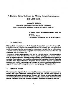
(a) settings for the trajectory

(b) 3D map

Fig. 1. In the left figure it is possible to change the depth of the vheicle and to define a trajectory given by interpolation of points. In the right figure, we can see the trajectory in the 3D scenario.

(i)

w(i) =

p(xt |z1:t , u0:t ) (i)

π(xt |z1:t , u0:t )

(3)

The weights w(i) account for the fact that the proposal distribution in general is not equal to the true distribution of the successor states. • Resampling: Particles with a low importance weight w are typically replaced by samples with a high weight. This step is necessary since only a finite number of particles are used to approximate a continuous distribution. Furthermore, resampling allows to apply a particle filter in situations in which the true distribution differs from the proposed one. The particle filter approach was chosen for multiple reasons. Firstly, it can handle estimation of non Gaussian and non linear processes. This is very important because nonlinearities are very frequent in AUVs, both in model specification and in the observation process. Additionally, noise cannot be modeled as Guassian in many situations. The second advantage in using particle filter is that it does not require any assumption on the initial position and orientation of the vehicle. However, the standard approach presents two main problems. The first one is the high number of particles required, in order to explore the state space, resulting in an increase of the computational power needed. The other major issue in particle filter approaches is the sample impoverishment problem, i.e. the loss of diversity for the particles to adequately represent the solution space [16]. In our approach, we address both these problems. With the proposed modification to the standard algorithm, it is possible to instantiate very few particles and, at the same time, assuring convergence to the correct state estimation, effectively exploring the solution space. The modification we propose in this paper is to instantiate during each step a portion of random particles. Thus, the resampling algorithm is now built with two modules. The first one is a standard SIR module, returning N − k particles. The second module returns k particles, created randomly. The combination

of these two modules constitute our proposal for the resampling step. In this way, after some time, the algorithm is able to recover in case of a wrong convergence, as shown in the following section. The standard particle filter algorithm is not able to do that, as the posterior is only dependent on the prior. The benefits on the computational point of view are relevant. There is no need anymore to instantiate the particles in order to cover all the state space. Even if in the initial step there are no particles near the real position of the vehicle, the proposed solution is still able to find the right state, after some time. A significant issue is to determine the optimal value of k. We have chosen an empirical approach, considering both map complexity and initial distribution of the particles. We found that a good system is to add at each step 1/5 of new particles, with 30% probability. III. S IMULATED SETUP The first step in the validation of the proposed approach is by simulation. Our system can model a vehicle with six degrees of freedom (DOF), plus a DOF for the mounting of the sensor on the sway axis. In this particular setup we have assumed that pitch and roll of the vehicle are neglected. Additionally, at this point, the sensor orientation in relation to the vehicle is fixed. A simulated gyroscope is used to have a noisy estimation of the orientation of the vehicle (yaw). A simulated depth sensor provides a noisy estimation of the distance between the vehicle and the seabed. Finally, a simulated profiling sonar is modelled to acquire range profiles. It is assumed that an a-priori map of the vehicle’s surroundings is known. No assumptions are made on the initial position of the vehicle within the map. The particle state is represented by six variables, three for orientation and three for position of the vehicle, plus an additional variable representing the weight of the particle. A synthetic environment was created to validate the approach. Different types of scenarios were considered, in order to analyze the algorithm performances.

Fig. 2. A 2D plot of the environment, with real trajectory (blue) and expected trajectories, given by particle analysis. The green (light gray) dot trajectory is given by the mean of the particles, while the red (dark gray) dash one is given by the best particle. The real trajectory starts at the beginning of the blue (black) line, on the top right of the figure. The particles in their last configuration are also shown, at the end of the trajectories, on the bottom center of the figure.

After defining an underwater scenario, a non linear trajectory is defined around the scenario, as shown in Fig. 1. To determine the expected position of the vehicle and, therefore, the expected trajectory, we consider two different possibilities: the weighted average of the particles and the best particle. Each solution has advantages and disadvantages. Choosing the average results in a smoother trajectory, but usually noisier. The best particle trajectory is much more dynamical, as it can jump from one particle to another one, in the first phase of the algorithm. As soon as a convergence is reached, the best particle trajectory presents a better overlapping of the real trajectory. In Fig. 2, the results of the simulation are presented in a 2D projection for more clarity, as all the trajectories tested are 3D. The contour of the environment is added to understand the trajectory according the environmenet at the vehicle position. The real trajectory is plotted in blue (black). The expected trajectories, given by particle analysis are plotted in green (light gray) and in red (dark gray). The green dot trajectory is given by the mean of the particles and the red dash trajectory is given by the best particle. As the figure shows, at the beginning, the inferred trajectories are not close to the real trajectory, because no assumptions are made on the initial position of the vehicle within the map. After a short time, the particles converge near the real position and they do not lose it. The figure shows the particles distribution at the last step, plotted according to their weight. Particles near the real trajectory are bigger than particle with a low weight. Fig. 3 shows the error between the real trajectory and the trajectories inferred by the particles. The green (light gray) dot error line is referred to the trajectory given by the mean of the particles, whilst the red (dark gray) dash error line is

Fig. 3. Simulated results: error between real trajectory and expected trajectories, inferred by the particles. The red (dark gray) dash error line is given by the best particle trajectory, while the green (light gray) dot error line is given by the mean trajectory.

referred to the trajectory given by the best particle. Before the convergence, the red (dark gray) dash line error is much more variable than the green (light gray) dot line error. That is because the trajectory given by the weighted average of the particle is much smoother, in this phase, than the trajectory given by the best particle, which is much more dynamical. In this situation, the red (dark gray) dash line error is usually greater than the green (light gray) dot line error. As soon as there is the convergence to the right position, the red (dark gray) dash line error is closer to zero than the green (light gray) dot line error is, providing a better estimation. After the convergence, the total red (dark gray) line error, represented by the integral of the error, is always lower than the green line error and, if we consider the actual error at any fixed time after the convergence, in more than 90% of cases. Evaluation on convergence shows that in 100% of tests, the red (dark gray) dash line error goes close to zero faster than the green (light gray) dot line error. This is expected, because the green (light gray) dot trajectory is affected by all the particles and needs some more resampling steps in order to discard the particles not representing a good estimation of the state and to converge to the real position. Fig. 4 shows an example of recovering from wrong convergence. At the beginning there is a convergence on the bottom of the map, as the structure is perceived by the vehicle similar to the sensor data from the sonar. However, as soon as the process evolves, it is able to recognize that the expected sensor measure is too far from the real one. Spreading k new random particles helps the vehicle to exit from local minima. In Fig. 5 the error graph is plotted. As explained before, the first trajectory to go close to the real one is given by the best particle trajectory. It is possible to see it in Fig. 4 (b), in which the expected position given by the best particle is very close to the real position, while the expected position given by the weighted average is far away, as it is influenced by the other particles not yet converged.

(a)

(b)

(c)

Fig. 4. 2D plot. Real trajectory is a solid blue (black) line, trajectory given by the best particle is a dash red (dark gray) line and trajectory given by the mean is a dot green (light gray) line; (a) Wrong particle convergence on the bottom of the figure. The real position is the blue circle on the blue trajectory on the top right of the figure; (b) recovering from the wrong convergence: the best particle expected position is very near the real position, while the mean expected position is still far, at about the center of the figure; (c) after the recovering, the particles are keeping the right position.

Fig. 5. Simulated results, recovery from wrong convergence: error between real trajectory and expected trajectories, inferred by the particles. The error is high and costant when the particles converge to a wrong position, but it goes close to zero as soon as the algorithm recovers. The red (dark gray) dash error line is given by the best particle trajectory, while the green (light gray) dot error line is given by the mean trajectory.

IV. E XPERIMENTAL RESULTS The robotic platform used for the experiments is a hover capable AUV such as the one in Fig. 6. The results presented in this section show the robustness of the proposed algorithm and its capability to be used in real missions. The trials were performed in a cylinder tank, 8 metres tall, with a diameter of 14 metres. The first part of our validation process was to test the localization algorithm in the empty tank, using the wall as a reference. After validating this first step, we added a cylindric metallic object in the center of the tank in order to analyze the performances of the algorithm adding some complexity to the environment. The assumptions for the real scenario are the same as for the synthetic one. An a-priori map of the vehicle surroundings is known. The vehicle is equipped with a fiber optical gyroscope, DVL and depth sensor, as proprioceptive sensors. A Tritech Seaking mechanically scanned profiling sonar is the main

Fig. 6.

The autonomous underwater vehicle RAUVER

exteroceptive sensor which acquires range profiles of the environment. In order to use our particle filter approach, we created a simulation of the sensor’s view as if the vehicle were located at each of the particle’s position. According to the particular geometrical situation of our test facility, we implemented a mathematical approach, in order to simulate the sensor data, possible because both the tank and the inner object are cylinders. Other approaches, such as ray tracing, are of course possible, but more computational expensive. In Fig. 7, a 2D plot with the initial particle distribution is presented. In Fig. 8, the expected trajectories are plotted, as well as the final configuration of the particles. The green (light gray) trajectory is given by the mean of the particles and the red (dark gray) trajectory is given by the best particle. The general behavior of the algorithm is the same both with real experiments and in simulation. There is some uncertainty at the beginning, but the particles converge to the right position quite quickly. The mission was to track the cylinder object,

Fig. 7.

Initial distribution of particles

Fig. 9. Trials with real vehicle: error between real trajectory and expected trajectories, inferred by the particles. The red (dark gray) dash error line is given by the best particle trajectory, while the green (light gray) dot error line is given by the mean trajectory.

before a new sonar picture is available. Using 40 particles, there is enough time for at least 5 steps, before adding the process evolution and starting analyzing the new sensor data. This results in a more accurate and precise localization. V. C ONCLUSION

Fig. 8. A 2D plot of the environment, with the particles, in their last configuration and with the expected trajectories, given by particle analysis. The green (light gray) dot trajectory is given by the mean of the particles, while the red (dark gray) dash one is given by the best particle.

keeping a fixed distance from it, for about a quarter of a complete turn and then come back on the same trajectory. As shown in Fig. 8, the proposed algorithm succesfully returns the expected trajectory for the described mission. Figure 9 shows the error between the real trajectory and the trajectories inferred by the particles. The green (light gray) dot error line is referred to the trajectory given by the mean of the particles, whilst the red (dark gray) dash error line is referred to the trajectory given by the best particle. The results are really good, even better than expected. In all our tests, the error is less than 40 cm, after the convergence. If we compare these results with the simulated data, they appear to be better. In reality, two factors have an impact on these results. As first, the complexity of the map has to be taken into account. The synthetic environment was much more complex and bigger than the real one, presenting similar profiles, which could lead more easily to a wrong convergence. Additionally, because of our efficient geometrical approach in analyzing the real data, it is possible to run multiple times the localization algorithm,

This paper has presented a particle filter approach for localization of autonomous underwater vehicles both in structured and unstructured environments. The paper has detailed the localization algorithm, as well as simulation and real experimental setup. Experimental results show the high performances of this algorithm, which is robust to noisy measurements. Future work is to integrate this algorithm in a docking mission. The proposed approach will be used as the module to localize the AUV position with respect to the docking station and to navigate to it. Extensions for the proposed approach include the assumption of a partially known map, with the integration of scan matching techniques. ACKNOWLEDGMENT This research was sponsored by the Marie Curie Research Training Network F REEsub N ET , Contract Number: MRTN−CT−2006−036186. The authors would like to thank all the staff both of OSL and SeeByte for their help, advice and support. R EFERENCES [1] J. Borenstein, H. R. Everett, L. Feng, and D. Wehe, “Mobile robot positioning: Sensors and techniques,” Journal of Robotic Systems, vol. 14, pp. 231–249, 1997. [2] E. Mouaddib and B. Marhic, “Geometrical matching for mobile robot localization,” IEEE Transactions on Robotics and Automation, vol. 16, no. 5, pp. 542–552, 2000. [3] K. Sutherland and W. Thompson, “Localizing in unstructured environments: dealing with the errors,” IEEE Transactions on Robotics and Automation, vol. 10, no. 6, pp. 740–754, 1994. [4] J. S. Stambaugh and R. B. Thibault, “Navigation requirements for autonomous underwater vehicles,” Navigation, 1992.

[5] M. Carreras, P. Ridao, R. Garcia, and T. Nicosevici, “Vision-based localization of an underwater robot in a structured environment,” Robotics and Automation, 2003. Proceedings. ICRA ’03. IEEE International Conference on, vol. 1, pp. 971 – 976, 2003. [6] A. Caiti, A. Garulli, F. Livide, and D. Prattichizzo, “Localization of autonomous underwater vehicles by floating acoustic buoys: a setmembership approach,” Oceanic Engineering, IEEE Journal of, vol. 30, no. 1, pp. 140–152, Jan. 2005. [7] M. Erol, L. Vieira, and M. Gerla, “Auv-aided localization for underwater sensor networks,” Wireless Algorithms, Systems and Applications, 2007. WASA 2007. International Conference on, pp. 44–54, Aug. 2007. [8] J. Kong, J. hong Cui, D. Wu, and M. Gerla, “Building underwater ad-hoc networks and sensor networks for large scale realtime aquatic applications.” in IEEE MILCOM, Atlantic City, NJ, USA,, 2005, pp. 1535 – 1541. [9] L. Collin, S. Azou, K. Yao, and G. Burel, “On spatial uncertainty in a surface long base-line positioning system,” in Proc. 5th Europ. Conf. Underwater Acoustics, Lyon, France, 2000. [10] N. Storkensen, J. Kristensen, A. Indreeide, J. Seim, and T. Glancy, “Huginuuv for seabed survey,” Sea Technol., 1998. [11] R. Karlsson, F. Gusfafsson, and T. Karlsson, “Particle filtering and cramer-rao lower bound for underwater navigation,” vol. 6, April 2003, pp. VI–65–8 vol.6. [12] S. Wirth, A. Ortiz, D. Paulus, and G. Oliver, “Using particle filters for autonomous underwater cable tracking,” in NGCUV’08, Killaloe, Ireland, 2008. [13] N. Gordon, D. Salmond, and C. Ewing, “A novell approach to nonlinear nongaussian bayesian estimation,” in Radar and Signal Processing, IEE Proceedings F, 1993. [14] A. Doucet, S. Godsill, and C. Andrieu, “On sequential monte carlo sampling methods for bayesian filtering,” Statist. Comput., vol. 10, pp. 197–208, 2000. [15] W. Burgard, D. Fox, and S. Thrun., “Robust monte carlo localization fot mobile robots,” Journal of Artificial Intelligence, 2001. [16] J. Carpenter, P. Clifford, and P. Fearnhead, “Improved particle filter for nonlinear problems,” Radar, Sonar and Navigation, IEE Proceedings -, vol. 146, no. 1, pp. 2–7, Feb 1999.