Hindawi Publishing Corporation Journal of Sensors Volume 2016, Article ID 2672640, 15 pages http://dx.doi.org/10.1155/2016/2672640
Research Article Bayesian Train Localization with Particle Filter, Loosely Coupled GNSS, IMU, and a Track Map Oliver Heirich DLR (German Aerospace Center), Institute of Communications and Navigation, 82234 Oberpfaffenhofen, Germany Correspondence should be addressed to Oliver Heirich;
[email protected] Received 23 October 2015; Revised 5 February 2016; Accepted 24 March 2016 Academic Editor: Yassine Ruichek Copyright © 2016 Oliver Heirich. This is an open access article distributed under the Creative Commons Attribution License, which permits unrestricted use, distribution, and reproduction in any medium, provided the original work is properly cited. Train localization is safety-critical and therefore the approach requires a continuous availability and a track-selective accuracy. A probabilistic approach is followed up in order to cope with multiple sensors, measurement errors, imprecise information, and hidden variables as the topological position within the track network. The nonlinear estimation of the train localization posterior is addressed with a novel Rao-Blackwellized particle filter (RBPF) approach. There, embedded Kalman filters estimate certain linear state variables while the particle distribution can cope with the nonlinear cases of parallel tracks and switch scenarios. The train localization algorithm is further based on a track map and measurements from a Global Navigation Satellite System (GNSS) receiver and an inertial measurement unit (IMU). The GNSS integration is loosely coupled and the IMU integration is achieved without the common strapdown approach and suitable for low-cost IMUs. The implementation is evaluated with real measurements from a regional train at regular passenger service over 230 km of tracks with 107 split switches and parallel track scenarios of 58.5 km. The approach is analyzed with labeled data by means of ground truth of the traveled switch way. Track selectivity results reach 99.3% over parallel track scenarios and 97.2% of correctly resolved switch ways.
1. Introduction Train localization inside a railway network is necessary for a collision-free operation and mainly addressed by centralized traffic control, signaling, and sensors in the railway infrastructure. Onboard train localization in combination with communications enables distributed and train centric assistant systems such as collision avoidance, coupling, and autonomous train operation. This localization system concept focuses on exclusive onboard computation and sensors without any additional railway infrastructure. Future railway systems such as a train centric collision avoidance system [1, 2] require a localization system with continuous availability and a track-selective accuracy. Track selectivity is the ability to identify the correct track, especially in the critical, parallel track scenario after a ride on a divisive switch way. The track selectivity is the technical challenge and also the major requirement of train localization. The goal of train localization is to determine the position of the train in the track network by topological coordinates, which are hidden variables and cannot be measured directly.
Single sensor systems, such as global navigation satellite systems (GNSS), are very beneficial for localization, but the measurement accuracy and lack of availability in parts of the railway environment do not fulfill the safety-critical requirements. Research on train localization with onboard sensors focuses on the following question: how is a train-borne, safety-critical, and onboard localization system designed and analyzed in terms of data processing with continuous availability and a track-selective accuracy? The approach should cope with hidden variables as the topological position, imprecise information of measurements from multiple sensor sources, outages, statistical noise, and systematic measurement errors. This paper presents a train localization approach by a Rao-Blackwellized particle filter (RBPF). Figure 1 shows the setup with onboard sensor data of an inertial measurement unit (IMU) and a GNSS receiver. The RBPF estimates the linear state variables of the one-dimensional train transition with Kalman filters within each particle of a particle filter. Furthermore, a novel empirical evaluation methodology
2
Journal of Sensors
GNSS Track map IMU
Sequential Bayesian filter
Track ID, track position, train frame direction, train speed
(i) Collision avoidance (ii) Speed monitoring (iii) Radio (iv) Train control
Figure 1: Bayesian train localization setup with GNSS, IMU, and a track map.
is defined for track selectivity which is not specific to a certain train localization approach. This paper is considered as a follow-up of the theoretic probabilistic approach with a particle filter [3–5] using satellite range measurements. The novel parts are the extension of the particle filter for train localization with a Rao-Blackwellization as well as an evaluation framework for track selectivity. The RBPF and a reference map-match approach are evaluated in terms of track-selective accuracy with real train data of a regional train. The outline of this paper starts with a related work review, a general information for a map-based train localization in Section 3, and the description of the used sensors in Section 4. Section 5 contains the derivation of the Rao-Blackwellization and the RBPF implementation is given in Section 6. The track-selective evaluation (Section 7) evaluates the RBPF approach with data from train runs (Section 8). Sections 9 and 10 show the results and the discussions on results.
2. Related Work There are multiple approaches of train localization in the literature with onboard sensors and a map. A selection of studies are chosen, which focus on track selectivity or specific sensor studies, which can identify the switch way. The different approaches vary in sensor types or combinations, processing methods, and evaluation scope and will be presented in these categories. Inertial sensors are often used in combination with an integrated navigation system for GNSS position aiding, for example, in [6, 7]. The yaw turn rate can also be used for the switch way identification that has been used in [8, 9] and analyzed in [10, 11]. Approaches with GNSS and IMU are found in [7–9] and extensions with eddy current sensor in [6, 12, 13]. The eddy current sensor, in principle a metal detector for characteristic railway features, can be used for a switch way detection, as speed or displacement sensor. Sensors such as cameras [14, 15] or LIDAR [16, 17] can directly identify the different switch ways and contribute to the trackselective result. A study of a tightly coupled localization with raw GNSS data and a track map was shown in [5, 18]. A tightly coupled approach considers pseudorange, Doppler, and phase measurements and has the advantage to process location information even with less than four satellites in view. However, a tightly coupled approach is typically more complex to implement than a loosely coupled approach and a user clock offset needs to be estimated additionally. The processing methods of each study are different and dependent
on the used sensors, filtering method, and algorithmic integration of the map. Saab proposed a train localization using a map-matching technique with a correlation of the curvature signature [19]. For the track selectivity, there are two classes with map integration and estimation of importance: a multiple hypothesis filter handles and maintains multiple estimates on several tracks in the vicinity and is commonly used [6, 9, 13, 17]. The particle filter uses usually a large set of particles, which are location hypotheses on a map, and handles the different track hypotheses by particles. The particle filter with onboard sensors and a map was proposed in [20]. Fouque and Bonnifait [18] defined a marginalized particle filter with raw GNSS data for the identification of the carriageway and along position of a road vehicle. Hensel et al. [12] showed a particle filter approach for railways based on just an eddy current sensor and a map. Only few approaches evaluate data sets with statistics about track selectivity: Lauer and Stein [13] used GNSS and a velocity sensor and showed a gain in track-selective accuracy and confidence between a simple map-match and a proposed estimation algorithm. Hensel et al. [12] showed no direct figures on switch way resolution but improved switch detection (98.23%) and classification (99.64%) with an eddy current sensor of 861 switches. This study focused on switches as position input and classifications on merging and splitting switch runs. B¨ohringer [6] evaluated an integrated navigation system (GNSS, IMU) in combination with an eddy current sensor for switch way identification. Even with a moderate switch detection rate of 70%, the results received 99.78% of track-selective accuracy. These results are considered as most suitable for a comparison and are based on real train runs of 120 km with 113 switches.
3. Map-Based Railway Navigation 3.1. Topological Coordinates. The goal of train localization is to estimate the train position in the track network by topological coordinates as well as the train speed V. A unique and discrete track ID (𝑖𝑑) identifies the track and the track length variable 𝑠 is the one-dimensional position on that track. Each track has an origin and a direction 𝑑𝑖𝑟 indicates if a train is oriented with or against the track definition. The topological coordinates are 𝑇topo = {𝑖𝑑, 𝑠, 𝑑𝑖𝑟} .
(1)
Tracks are connected by switches, crossings, or diamond switch crossings. A track 𝑖𝑑 is defined between connections with a unique ID; that is, it contains no switch or
Journal of Sensors
3 Table 1: Train directions.
Train-track frame direction 𝑑𝑖𝑟
Train velocity direction 𝑚 = sign (V)
Train-track frame motion direction sign (𝑠)̇
+ − + − + −
Forward (+) Forward (+) Backward (−) Backward (−) Stop (0) Stop (0)
+ − − + 0 0
crossing. This definition ensures that a track 𝑖𝑑 is always one-dimensional and limited by the two endings of track beginning and track end. 3.2. Coordinate Frames. The sensors measure in their specific sensor frame. For further processing, these measurements are converted in the train frame according to the mounting parameters. The map and especially the geometry of the tracks are expressed in the track frame. Any sample point of a track contains a geographic position (WGS84) and the track attitude angles are defined from a local frame in north, east, and down (NED). Once angles or curvatures are used in the map, there is an ambiguity about the direction at which the track ending the origin is defined. Therefore, it is necessary to define a start point and consequently a pointing direction of the track. A train (train frame) can be placed in two orientations on a track and can move forward or backwards. Alternatively to V, the train speed can be expressed between train and track frame by 𝑠.̇ The absolute velocities of V and 𝑠̇ are the same. The sign of 𝑠̇ indicates either an increasing (+) or decreasing (−) change of the position 𝑠 of the current track and depends on the track definitions. Throughout this approach, the map information of a specific location is converted and processed in the train frame. It should be noted that there is an alternative way to convert all variables to the track frame. Table 1 shows the conversions of the train direction variables: train-to-track frame direction (𝑑𝑖𝑟), the motion direction of the train (𝑚), and the direction of motion between train and track frame by the sign of 𝑠.̇ The motion direction 𝑚 depends on a forward or backward velocity V regarding the train frame definition of front and rear. It is possible to compute any of these directions from the two others by Table 1. Direction 𝑑𝑖𝑟 keeps its value during standstill. The motion direction 𝑚 remains the same during a train run, while the sign of 𝑠̇ and 𝑑𝑖𝑟 can alternate after a change of tracks during a train run. 3.3. Along Track and Cross Track. A suitable analysis for topological localization performance is the approach by along and cross track. Along track addresses the continuous 1D localization on a track. Cross track focuses on discrete, different tracks and track selectivity is the ability of a correct cross track localization. Sensors can contribute to along and cross localization with relative or absolute measurements of displacement or track features. As shown in Figure 2,
Cross at switch (idleft , idright )
Absolute along (s)
Realtive along (Δs)
Absolute cross (id)
Figure 2: Along and cross track definitions.
measurements can contribute to train localization in four different ways: (i) relative along (Δ𝑠): odometry, (ii) absolute along (𝑠): diverse along-track features, (iii) cross at switch (𝑖𝑑): competing switch way track features, (iv) absolute cross (𝑖𝑑): diverse cross/parallel track features. Odometry is the processing of relative along measurements, such as wheel turns, speed, and train acceleration. Depending on track features, parallel tracks show often very similar along and cross track features. Measurements may contribute to absolute along or cross in a local vicinity or even globally. 3.4. Railway Track Features. A suitable track feature is an unchanging property of the track which can be measured by a sensor. Over different locations, there are unique track features as well as repeated, ambiguous features possible. Here, the features are the track geometry by geographic position (latitude 𝜑, longitude 𝜆), track attitude (i.e., heading 𝜓), and curvature. The heading 𝜓(𝑠) changes over the run of the track, which is represented by the heading curvature 𝑐𝜓 = 𝑑𝜓(𝑠)/𝑑𝑠. Additional features can be extended, provided that there is a reproducible signal over different locations and sensors can measure these features. 3.5. Railway Switch. The switch way identification is a critical process in railway navigation, especially if the tracks are parallel after the train passes a splitting switch. As a special property of a switch, the two tracks of the competing switch ways differ in geometric characteristics of curvatures 𝑐𝜓 , headings 𝜓, and geopositions (latitude 𝜑, longitude 𝜆). The geopositions of left and right switch way are located apart by the cross track distance 𝑑CT . The switch way track positions and headings increase slowly from the switch start, while the curvature is already present from the switch start. There can be many more switch way features, as shown in other approaches based on different sensors [12]. 3.6. Track Map. The railway map works as a coordinate transformation between topological coordinates and track features (e.g., geometric coordinates). The map model contains and connects information on topology and track features. These track features are parametrized by the 1D-position 𝑠 and stored in discrete points (track points). A continuous representation of track features is achieved by interpolations
4
Journal of Sensors
between these points. The track features can be obtained from the map by the topological pose and converted to train frame: { 𝜓 } ̂ ⏟⏟ , ⏟⏟⏟̂𝑐⏟⏟ ⏟⏟ } 𝑓map (𝑖𝑑, 𝑠, 𝑑𝑖𝑟) = { ⏟⏟𝜑, ⏟⏟ ⏟⏟⏟𝜆⏟⏟ , ⏟⏟⏟𝜓 curvature geo position attitude } {
train
.
(2)
According to the train direction 𝑑𝑖𝑟, the sign of the curvature 𝑐𝜓 changes, while 𝜓 changes by 180∘ . This special map can be constructed from train-side sensor data [7, 21] or extracted from an existing geodatabase. An open street map (OSM) [22] geodatabase is used as data source for the track map. The main advantages of OSM are the availability and the completeness of data points of many tracks of the desired railway track network. For an adequate map, there is some additional preparation by track separation and topological connection (e.g., at switches) as well as geometry processing being necessary. An OSM data contains geodata points (𝜑, 𝜆) and the track geometry of heading (𝜓) and heading curvature (𝑐𝜓 ) is derived from these positions. The data is usually collected from various sources, such as a GNSS hand-held or extracted from aerial or satellite photo with different and undefined accuracy. Therefore, an OSM data based map should not be considered as highly accurate. An analysis of many train runs showed lateral deviations up to 5 m between an averaged GNSS trace and the OSM track. 3.7. Train State Estimation. The estimation state of railway localization is formulated with the following random variables: (i) track ID: 𝑖𝑑 (discrete),
The strong track-train constraint allows to predict the train position, attitude, and inertial state from the known track geometry of the map. These extended train states are computed from the map by the actual topological position estimate and contains the geometry in train frame (𝜓 and 𝑐𝜓 transformation according to 𝑑𝑖𝑟): ̂ , ̂𝑐𝜓 }𝑘 𝑇𝑘ext = {𝜑, 𝜆, 𝜓
train
.
(5)
3.8. Train Control. The train control consists of cross track control and the along-track control by the train driver: } { } { } { sw ⏟⏟ , ⏟⏟⏟⏟⏟⏟⏟⏟⏟⏟⏟⏟⏟⏟⏟ 𝑈acc , 𝑈𝑚 } . 𝑈 = { ⏟⏟𝑈⏟⏟⏟ { } { cross control, along control, } { control center train driver }
(6)
The cross control influences the travel path of the train by the selected switch way (𝑈sw : {left, right}). This is usually controlled by a train control center or sometimes by the train driver at shunting yards or industrial tracks. The train driver controls the general train motion 𝑈𝑚 and the acceleration 𝑈acc by the traction and brake lever. The general train motion is the travel direction selector as well as a train stop (e.g., activated parking brakes). The control center has also influence on the along-track control via signaling. 3.9. Simple Map-Matching. In contrast to state estimation a reference approach by simple map-matching is described. The simple map-matching is a snapshot based, nearest neighbor method, which uses no information about the prior position. The nearest position on track is computed with the map from a GNSS position measurement:
(ii) position: 𝑠 (continuous, only within a track), (iii) train direction on track: 𝑑𝑖𝑟 (binary),
{𝑖𝑑, 𝑠} ⏟⏟⏟⏟⏟⏟⏟⏟⏟
(iv) train speed: V (continuous),
topo position
(v) train acceleration: 𝑎 (continuous), (vi) correlated sensor properties: biases: 𝑏 (continuous). The estimation state vector or train state 𝑇𝑘est for one discrete time step 𝑘 is defined by } { 𝑇𝑘est = { ⏟⏟⏟⏟⏟⏟⏟⏟⏟⏟⏟⏟⏟⏟⏟ 𝑖𝑑, 𝑠, 𝑑𝑖𝑟 , ⏟⏟V, ⏟⏟⏟𝑎⏟⏟ } . {topological pose train motion}𝑘
(3)
The train-to-track frame speed 𝑠̇ can be computed by Table 1: {V 𝑘 , 𝑠𝑘̇ = { −V , { 𝑘
if 𝑑𝑖𝑟 = +, if 𝑑𝑖𝑟 = −.
(4)
The bias vector 𝐵𝑘 contains correlated sensor errors. These biases change over time due to a random drift, which cannot be calibrated in advance. Additionally to the state variables, an auxiliary variable 𝑚 is used to represent the vehicle motion by 𝑚 ∈ {forward, stop, backward}. The goal for a train localization algorithm is to estimate and resolve 𝑇𝑘est and 𝐵𝑘 .
= 𝑓map-match ( ⏟⏟𝜑, ⏟⏟⏟𝜆⏟⏟ ) .
(7)
geo position
It should be noted that this approach would be sufficient if the position measurement (e.g., ideal GNSS) is continuously available with an accuracy always better than half of the distance of parallel tracks. It will be shown in the results that this approach has its problems with real GNSS position measurements.
4. Train-Side Sensor Measurements This paper focuses only on GNSS and IMU measurements, but other train-born sensors can extend the proposed approach. The used sensors are considered as inexpensive and their combination as complementary in terms of measurement errors. 4.1. Global Navigation Satellite Systems. The approach uses the standard GNSS receiver output by position-velocity-time (PVT) and is considered as loosely coupled. That means that the internal GNSS related computations can be kept transparent, up-to-date with actual receiver technology and out of the train localization approach. The used receiver was
Journal of Sensors
5
a u-blox 6 GPS receiver, but also other commercial off-theshelf receivers could be used. A drawback of GNSS is the lack of availability and degraded accuracy in parts of the railway environment. GNSS data is not available in tunnels or below station roofs. The accuracy is further affected by multipath, signal loss, and poor geometry in urban environments, next to acoustic noise barriers or in dense forests.
with single antenna is the heading of the antenna motion and requires a conversion to train frame by the train motion 𝑚 (see also Table 1):
4.1.1. GNSS Speed. The GNSS speed measurement contributes to the train odometry in terms of relative along-track estimation and is part of the PVT data. A single antenna mounting is invariant of a horizontal rotation; that is, the speed and also heading measurements are independent of the mounted yaw angle between antenna and train. In principle, the GNSS speed is computed from the vector norm of the antenna motion in north and east component. Therefore, the GNSS speed is always positive and the train motion (𝑚) must be considered in the use-case for train speed. The measurement model contains the train speed 𝑠,̇ additional white noise 𝑛, and a conversion for the train motion:
It should be noted that there are no heading measurements for very low speeds or stopped trains.
V {−V𝑘 + 𝑛𝑘 , 𝑍𝑘GNSS,V = { V + 𝑛𝑘V , { 𝑘
if 𝑚 = backwards, if 𝑚 = forwards.
(8)
4.1.2. GNSS Positions. GNSS positions are a favorable measurement for absolute along and cross resolution of the train location. The GNSS position model includes 2D positions of latitude 𝜑 and longitude 𝜆 and additional white noise 𝑛pos : GNSS,pos
𝑍𝑘
𝜑 pos = ( ) + 𝑛𝑘 . 𝜆 𝑘
(9)
4.1.3. GNSS Heading. The GNSS heading angle contributes to the switch resolution which was described as cross at switch contribution in Section 3.3. There are multiple ways of the internal heading computation of the receiver: a simple differentiation of two consecutive positions or by computation of a receiver motion vector from Doppler and/or phase measurements of each satellite. The actual internal method is unknown, but state-of-the-art methods use positions and Doppler within a Kalman filter [23]. The used receiver outputs an ECEF (earth centered, earth fixed) velocity vector, and the GNSS heading measurement is the angle to north of the horizontal part of this vector in east and north direction. The receiver estimates further an accuracy of the velocity vector (ECEF) better than 1.1 km/h in 95% of all runs and a resulting heading accuracy of 1.7∘ in 95% of all runs above 10 km/h. The GNSS heading is worse at low speeds, so the heading measurements are used above 10 km/h. The GPS data of the experiment and the results showed a good heading repeatability with usually less than 1∘ of different runs over the same positions. In comparison, a heading angle between two consecutive positions showed much worse results. The heading model contains the heading angle 𝜓 of the train (train frame) which is derived from the estimate of the topological pose and the map. A GNSS heading measurement
GNSS,𝜓
𝑍𝑘
̂ 𝑘 + 𝜋 + 𝑛𝑘𝜓 , if V < 0 (𝑚 = backwards) , {𝜓 ={ ̂ + 𝑛𝑘𝜓 , 𝜓 if forwards. { 𝑘
(10)
4.2. Inertial Sensor. The IMU measurements provide continuous and interference-free data. Two measurements are of particular interest: the longitudinal acceleration (𝑎𝑥 ) and the yaw turn rate (𝜔𝑧 ). The measurements are aligned with the train frame by prior calibration. 4.2.1. Longitudinal Acceleration. The longitudinal acceleration (𝑎𝑥 ) measures the train acceleration measurement and it contributes to the relative along localization (odometry). The along acceleration measurement model considers train acceleration 𝑎, the gravity 𝑔 portion by the slope angle 𝜃 of the track, and accelerometer bias 𝑏𝑎𝑥 : 𝑍𝑘IMU,𝑎𝑥 = 𝑎𝑘 + 𝑔 ⋅ sin 𝜃𝑘 + 𝑏𝑘𝑎𝑥 + 𝑛𝑘𝑎𝑥 . ⏟⏟⏟⏟⏟⏟⏟⏟⏟⏟⏟⏟⏟⏟⏟⏟⏟⏟⏟⏟⏟⏟⏟⏟⏟⏟⏟ ̃𝑏𝑘
(11)
Inertial sensors are affected by a bias which is changing over time, called drift. Any bias causes growing errors, as the train acceleration is integrated over time to speed and position. The presented approach does not contain a slope estimation or slope profile in the map. The slope angles of railway tracks are relatively small and the bias estimation in the following handles the difference. A continuous estimation of the combined offset ̃𝑏𝑘 is processed and contains bias and gravity portion from slope. Extensions with slope estimation by integration or a slope profile in the map are possible. 4.2.2. Yaw Turn Rate. Rails are a strong constraint between track geometry and train trajectory. It is possible to measure the geometric characteristics with a train-side IMU of a moving train. A certain curvature 𝑐𝜓 of a track causes yaw turn rates depending on the train speed: ̂𝑐𝜓 =
𝜓̇ . V
(12)
A complete model of train kinematics for turn rates and centripetal accelerations is presented in [21]. Trains are exposed to low pitch and roll angles in general and especially at switches. As a consequence, the horizontal heading turn rate 𝜓̇ can be approximated by the yaw rate of the train: 𝜓̇ ≈ 𝜔𝑧 .
(13)
The curvature as measurable track feature indicates absolute along locations and resolves different switch ways (cross at
6
Journal of Sensors
switch). This approach is less sensitive to drift as it does not rely on integration of the inertial measurements. This property is advantageous for the use of low-cost MEMS gyroscopes. The measurement model ℎ𝜔 of the yaw rate measurement 𝜔𝑧 is defined by 𝜓
𝑔𝑧
𝜔𝑧 𝑍𝑘IMU,𝜔𝑧 = ̂𝑐⏟⏟⏟⏟⏟⏟⏟⏟⏟⏟⏟⏟⏟⏟⏟⏟⏟⏟⏟⏟⏟ 𝑘 ⋅ V𝑘 + 𝑏𝑘 + 𝑛𝑘 . ℎ𝜔𝑧 (𝑇𝑘 ,𝐵𝑘 )
(14)
At this point, the frame and motion definitions are vital (Table 1). The curvature is translated to train frame by train direction 𝑑𝑖𝑟 and the speed contains the motion direction 𝑚 in its sign. The bias of the gyroscope (𝑏𝑔𝑧 ) is calibrated only during stop phases of the train: 𝑔𝑧
𝑏𝑘 ≈ 𝜔𝑧 ,
if 𝑚 = stop.
5.2. Along Track. One extension to the previous particle filter approaches [3, 4] is the separation of states, where certain states are estimated differently. In combination with particle filters, this process is called Rao-Blackwellization [24]. In particular the linear states can be separated from the nonlinear states of a particle hypotheses and estimated by a more optimal filter, as the Kalman filter. The train state contains linear and nonlinear parts: 𝑇𝑘 = {𝑇𝑘𝑙 , 𝑇𝑘𝑛 }. The train transition of 16 is split in a linear and nonlinear part via chain rule and conditional independencies that are removed: 𝑛 𝑙 , 𝑇𝑘−1 , 𝑈𝑘 , 𝑀) 𝑝 (𝑇𝑘 | 𝑇𝑘−1 , 𝑈𝑘 , 𝑀) = 𝑝 (𝑇𝑘𝑛 , 𝑇𝑘𝑙 | 𝑇𝑘−1 𝑛 , 𝑈𝑘 , 𝑀) = 𝑝 (𝑇𝑘𝑛 | 𝑇𝑘𝑙 , 𝑇𝑘−1 ⏟⏟⏟⏟⏟⏟⏟⏟⏟⏟⏟⏟⏟⏟⏟⏟⏟⏟⏟⏟⏟⏟⏟⏟⏟⏟⏟⏟⏟⏟⏟⏟⏟⏟⏟⏟⏟⏟⏟⏟⏟⏟⏟⏟⏟
(15)
nonlinear train transition on tracks
The turn rates are assumed to be zero and the low earth turn rate is neglected. The resulting small error is not integrated in the following (e.g., as in strapdown approaches) and results in a negligible error at the weighting process by a likelihood.
5. Probabilistic Train Localization The following definitions can be used for a multihypothesis filter, a particle filter or Rao-Blackwellized particle filter. The posterior is already specified for GNSS and IMU sensors. 5.1. Train Localization Posterior. The train localization posterior represents the estimation problem. In previous works [3, 4, 21], Bayesian methods are presented with a dynamic Bayesian network definition for the train localization problem and the factorization of the posterior is shown in steps. The posterior of all train states (𝑇0:𝑘 ) and sensor biases (𝐵0:𝑘 ) over 𝑘 time steps are estimated given all measurements (𝑍0:𝑘 ), train control inputs (𝑈0:𝑘 ), and the map (𝑀). The map is actually known in advance and does not change over time for the train localization problem. It is included in the conditional part of the distributions to indicate where information of the map is needed. The unknown train control is also included to indicate where a train driver or train control can influence the train states. The posterior is factorized in a recursive form in order to compute the posterior practically with estimation algorithms:
∝𝑝 (𝑍𝑘GNSS | 𝑇𝑘 ) ⋅ 𝑝 (𝑍𝑘IMU | 𝑇𝑘 , 𝐵𝑘 ) ⏟⏟⏟⏟⏟⏟⏟⏟⏟⏟⏟⏟⏟⏟⏟⏟⏟⏟⏟⏟⏟⏟⏟⏟⏟⏟⏟⏟⏟⏟⏟⏟⏟⏟⏟⏟⏟⏟⏟⏟⏟⏟⏟⏟⏟⏟⏟⏟⏟⏟⏟⏟⏟⏟⏟⏟⏟⏟⏟⏟⏟⏟⏟⏟⏟ measurements
⋅𝑝 (𝑇𝑘 | 𝑇𝑘−1 , 𝑈𝑘 , 𝑀) ⋅ 𝑝 (𝐵𝑘 | 𝐵𝑘−1 ) ⏟⏟⏟⏟⏟⏟⏟⏟⏟⏟⏟⏟⏟⏟⏟⏟⏟⏟⏟⏟⏟⏟⏟⏟⏟⏟⏟⏟⏟⏟⏟⏟⏟⏟⏟⏟⏟ ⏟⏟⏟⏟⏟⏟⏟⏟⏟⏟⏟⏟⏟⏟⏟⏟⏟⏟⏟⏟⏟⏟⏟ train transition
𝑙 ⋅ ⏟⏟⏟⏟⏟⏟⏟⏟⏟⏟⏟⏟⏟⏟⏟⏟⏟⏟⏟⏟⏟⏟⏟⏟⏟⏟⏟⏟⏟⏟⏟ 𝑝 (𝑇𝑘𝑙 | 𝑇𝑘−1 , 𝑈𝑘 ). linear train transition
5.2.1. Train Odometry Filter. The linear and one-dimensional train transition is separated from the nonlinear transition on the map and estimated with a Kalman filter. The estimation of the linear state variables of acceleration 𝑎, speed V, and displacement Δ𝑠 will be called odometry in the following. The odometry combines also the along acceleration bias estimation with updates from acceleration and speed measurements: 𝑙 ax , 𝑈𝑘 ) ⋅ 𝑝 (𝐵𝑘ax | 𝐵𝑘−1 ) 𝑝 (𝑇𝑘𝑙 | 𝑇𝑘−1 ⏟⏟⏟⏟⏟⏟⏟⏟⏟⏟⏟⏟⏟⏟⏟⏟⏟⏟⏟⏟⏟⏟⏟⏟⏟⏟⏟⏟⏟⏟⏟⏟⏟⏟⏟⏟⏟⏟⏟⏟⏟⏟⏟⏟⏟⏟⏟⏟⏟⏟⏟⏟⏟⏟⏟⏟⏟⏟⏟⏟⏟ odometry prediction
⋅𝑝 (𝑍𝑘GNSS,V | 𝑇𝑘𝑙 ) ⋅ 𝑝 (𝑍𝑘IMU,ax | 𝑇𝑘𝑙 , 𝐵𝑘ax ). ⏟⏟⏟⏟⏟⏟⏟⏟⏟⏟⏟⏟⏟⏟⏟⏟⏟⏟⏟⏟⏟⏟⏟⏟⏟⏟⏟⏟⏟⏟⏟⏟⏟⏟⏟⏟⏟⏟⏟⏟⏟⏟⏟⏟⏟⏟⏟⏟⏟⏟⏟⏟⏟⏟⏟⏟⏟⏟⏟⏟⏟⏟⏟⏟⏟⏟⏟⏟⏟⏟⏟⏟⏟
(16)
bias transition
⋅ ⏟⏟⏟⏟⏟⏟⏟⏟⏟⏟⏟⏟⏟⏟⏟⏟⏟⏟⏟⏟⏟⏟⏟⏟⏟⏟⏟⏟⏟⏟⏟⏟⏟⏟⏟⏟⏟⏟⏟⏟⏟⏟⏟⏟⏟⏟⏟⏟⏟⏟⏟⏟⏟⏟⏟⏟⏟⏟⏟⏟⏟⏟⏟⏟⏟ 𝑝 (𝑇0:𝑘−1 , 𝐵0:𝑘−1 | 𝑍1:𝑘−1 , 𝑈1:𝑘−1 , 𝑀). recursion
The factorized posterior is proportional (∝) to the posterior, because of a missing normalization factor. This normalization can be computed separately, as all probabilities sum up to one. There are different considerable filter approaches, which are able to estimate the nonlinear train transition and the different hypotheses of the topological pose.
(18)
odometry update
The state transition of the odometry prediction step is defined here as a 1D transition DWPA model (discrete white noise constant acceleration) [25]. The linear 1D train transition and the acceleration bias are estimated by the discrete model: Δ𝑡2 Δ𝑠 0 2 V V ( ) = (0 1 Δ𝑡 0) ( ) . 𝑎 𝑎 0 0 1 0 ̂𝑏 ̃𝑏 𝑘 𝑘−1 0 0 0 1) ( ⏟⏟⏟⏟⏟⏟⏟⏟⏟⏟⏟⏟⏟⏟⏟⏟⏟⏟⏟⏟⏟⏟⏟⏟⏟⏟⏟⏟⏟⏟⏟⏟⏟⏟⏟⏟⏟⏟⏟ Δ𝑠
𝑝 (𝑇0:𝑘 , 𝐵0:𝑘 | 𝑍1:𝑘 , 𝑈0:𝑘 𝑀)
(17)
0 Δ𝑡
(19)
system matrix
This model is propagated by state-of-the-art Kalman filter and updated with GNSS speed and longitudinal IMU acceleration measurements. 5.2.2. Track Transition Model. The track transition ensures that the estimates (hypotheses, particles) exist and stay exclusively on tracks. The nonlinear train transition of (17)
Journal of Sensors
7
estimates a topological coordinate from the linear displacement, the previous coordinate, an unknown switch way, and the map: 𝑝 (𝑇𝑘𝑛
|
𝑤𝑘 ∝
𝑛 𝑇𝑘𝑙 , 𝑇𝑘−1 , 𝑈𝑘 , 𝑀) topo
= 𝑝 (𝑇𝑘
topo
| 𝑇𝑘−1 , Δ𝑠𝑘 , 𝑈𝑘sw , 𝑀) .
topo
topo
= 𝑓map,trans. (𝑇𝑘−1 , Δ𝑠𝑘 ) .
topo
(22)
5.3. Cross Track. The cross track estimation evaluates different tracks at a switch or in scenarios with multiple tracks. The evaluation or weighting process is based on a soft comparison of measurements and expected measurements from the map. A sensor likelihood function is defined for each measurement type. First, the expected or estimated measurement is computed from a measurement model and the current state of train state and sensor correlation 𝑌𝑘 = ℎ(𝑇𝑘 , 𝐵𝑘 ). A generic likelihood function model is defined here with a Gaussian distribution. The mean is the expected measurement 𝑌𝑘 , the argument is 𝑍𝑘 , and the covariance of the sensor noise is Σ: 𝑝 (𝑍𝑘 | 𝑇𝑘 , 𝐵𝑘 ) 1 𝑇 = ̂ |2𝜋Σ|−1/2 exp {− (𝑍𝑘 − 𝑌𝑘 ) Σ−1 (𝑍𝑘 − 𝑌𝑘 ) } . 2
(23)
6. Particle Filter Approach A particle filter is chosen for the posterior (16) estimation. The particle filter can handle different nonlinear estimates (hypotheses) automatically by the particles, which is necessary for a distribution of any possible position over different tracks. As described in [26], a particle filter represents probability density functions by appropriate particle distributions with appropriate weights of 𝑁𝑝 particles. The posterior of (16) is represented by the particles set: 𝑁𝑝
𝑖 , 𝑤𝑖 }𝑖=1 . 𝑝 ({𝑇, 𝐵}0:𝑘 | 𝑍1:𝑘 , 𝑈0:𝑘 , 𝑀) ≈ {𝑥0:𝑘
(24)
𝑖 is the 𝑖th particle with its weight 𝑤𝑖 of 𝑁𝑝 particles and 𝑥0:𝑘 represents one sample of the posterior of all time steps until 𝑘. Particles are generated from a function which is easy to calculate [26], called the proposal function: 𝑖 ∼ 𝑞 ({𝑇, 𝐵}0:𝑘 | 𝑍1:𝑘 , 𝑈0:𝑘 , 𝑀) . 𝑥0:𝑘
𝑤, unnormalized weights
𝜂=
(21)
).
(26)
The weights of the particle filter sum up to one and the normalization factor 𝜂 can be easily computed:
This model considers the discontinuity at a track change and in case of a splitting switch scenario the next track is sampled from a discrete uniform distribution (left or right). According to the motion state of standstill (𝑚 = STOP), this transition can be suspended. The next step is a track map query by the topological pose for each hypotheses or particle. The extended train state 𝑇𝑘ext contains the track geometry in train frame: 𝑇𝑘ext = 𝑓map,data (𝑇𝑘
𝑝 ({𝑇, 𝐵}0:𝑘 | 𝑍1:𝑘 , 𝑈0:𝑘 , 𝑀) . 𝑞 ({𝑇, 𝐵}0:𝑘 | 𝑍1:𝑘 , 𝑈0:𝑘 , 𝑀) ⏟⏟⏟⏟⏟⏟⏟⏟⏟⏟⏟⏟⏟⏟⏟⏟⏟⏟⏟⏟⏟⏟⏟⏟⏟⏟⏟⏟⏟⏟⏟⏟⏟⏟⏟⏟⏟⏟⏟⏟⏟⏟⏟⏟⏟⏟⏟⏟⏟⏟⏟
(20)
The function of the map for each hypothesis (particle) is 𝑇𝑘
Afterward these particles are weighted [26]. The weights are proportional to the fraction posterior over proposal function:
(25)
1 𝑁𝑝 ∑𝑖=1
𝑤𝑖𝑘
.
(27)
After several time steps, some particles may carry an extreme high weight while the rest has a very low weight. These low weighted particles are inefficient and this process is called degeneration. In order to avoid this, a systematic resampling [26] of the particle distribution can solve this problem. A metric for particle depletion is the effective number of ̂ eff [25]. The particle distribution is resampled if particles 𝑁 ̂ 𝑁eff is below a threshold 𝑁th . 6.1. Particle Filter with GNSS and IMU Measurements 6.1.1. Proposal Function. The proposal function is designed by the transitions of train and correlated sensor properties as well as suitable measurements. The proposal contains the train odometry estimation of Section 5.2.1 and a gyroscope bias estimation. In this implementation, the gyroscope bias is only updated if the train is not moving. The displacement of the 𝑖th particle is sampled from the odometry Kalman filter output: 𝑖 2 , 𝜎Δ𝑠 ). Δ𝑠𝑘𝑖 ∼ N (Δ𝑠KF
(28)
In contrast to previous approaches [3, 4], the samples were directly generated from an acceleration distribution and a motion model. The use of the odometry Kalman filter inside of a particle filter is the Rao-Blackwellization part. The nonlinear map transition of (21) and map query (22) is processed for each particle as a function of the map. 6.1.2. Weight Function. The weight function is the combination of IMU and GPS likelihoods and computed as shown in (23) with the appropriate measurement models (9), (10), and (14). The weight function for the 𝑖th particle with the IMU and GNSS likelihoods is 𝑖 ⋅ 𝑝 (𝑍𝑘 𝑤𝑘𝑖 = 𝜂 ⋅ 𝑤𝑘−1
GNSS,pos
IMU,𝜔𝑧
⋅ 𝑝 (𝑍𝑘
| 𝑇𝑘𝑖 ) ⋅ 𝑝 (𝑍𝑘
GNSS,𝜓
| 𝑇𝑘𝑖 , 𝐵𝑘𝑖 ) .
| 𝑇𝑘𝑖 )
(29)
6.1.3. Initialization. The initial particle distribution is generated from the first GNSS position measurement. Therefore, the 2D geoposition is sampled 𝑁𝑝 times with a large covariance Σ (e.g., 100 m) from a Gaussian distribution: p̃ os𝑖 ∼ N (posGNSS 𝑘=1 , Σ) .
(30)
The positions are map-matched by (7) to topological positions and assigned to each particle 𝑖. The train frame direction 𝑑𝑖𝑟 is sampled randomly from a uniform distribution.
8
Journal of Sensors
6.2. Output Estimate. A particle distribution is a less useful output for applications like automated train control or collision avoidance. There, a single mode or most likely output is desired. Internally, the particle filter keeps its particle distribution for the next update. The output is computed by four steps: first, the track paths are identified and, second, the most likely track path with particles is chosen (ML path). A mean square estimate is computed from particles on that path and the result is translated back to topological coordinates. 6.2.1. Track Path Identification. At first, all path hypotheses 𝑖𝑑𝑝 with at least one particle are identified: 𝑁𝑝
𝑖 𝑖𝑑0:𝑗 𝑝 = 𝑓findPaths ({𝑖𝑑 }𝑖=1 ) .
6.2.2. ML Path. As a next step, the sum of weights are calculated for each path 𝑗: 𝑁𝑝
𝑖=1
selects weight of 𝑖th particle from the 𝑗th path 𝑖𝑑𝑝
(32)
The delta function 𝛿(𝑖𝑑𝑖 = 𝑖𝑑 ∈ 𝑖𝑑𝑗𝑝 ) equals one if the 𝑖th particle (respective its track ID 𝑖𝑑) is on the 𝑗th track path and is zero otherwise. The most likely path 𝑖𝑑ML 𝑝 is the path ML ̂ : index 𝐽 with the highest cumulative weight 𝑤 𝑤𝑗 ) . 𝐽 = 𝑓arg max 𝑗 (̂
(33)
6.2.3. Mean Square Estimate on Path. In the following, a delta function selects the 𝑖th particle which is on the most likely path: 𝛿𝑖 = 𝛿 (𝑖𝑑𝑖 = 𝑖𝑑 ∈ 𝑖𝑑ML 𝑝 ).
(34)
The topological coordinates of the selected particles are translated to the most likely path: topo,𝑖 ̃ =𝑓 ̃ topo,𝑖 : {𝑖𝑑, ̃𝑠, 𝑑𝑖𝑟} 𝑇 , 𝑖𝑑𝑝 ) . topo2path (𝑇
(35)
The 1D position is calculated by a weighted mean of the selected particles, which belong to the ML path: 𝑁𝑝
̂𝑠 =
1 ∑ (̃𝑠𝑖 ⋅ 𝑤𝑖 ⋅ 𝛿𝑖 ) . ̂ML 𝑖=1 𝑤
̂𝑠 = √ 𝜎
(36)
𝑁𝑝
2 1 ∑ ((̃𝑠 𝑖 − ̂𝑠) ⋅ 𝑤𝑖 ⋅ 𝛿𝑖 ). ̂ML 𝑖=1 𝑤
(37)
The train direction on track 𝑑𝑖𝑟 is computed by the highest weight, where 𝑙 is either positive or negative track frame direction of the path: ̂ML,+ = 𝑤
(31)
A track path contains one or more sequential tracks (𝑖𝑑) on a 1D path, where a train is able to run over in a sequence. For further computations, a track path has a continuous 1D coordinate frame compared to discontinuities at the joints of tracks. A topological pose can be translated into path coordinates as well as translated from path coordinates. As an example, in case of a split switch scenario, particles can be distributed before the switch, on the left and right switch way. This would result in two possible track paths: 𝑖𝑑1𝑝 = {𝑖𝑑before , 𝑖𝑑left } and 𝑖𝑑2𝑝 = {𝑖𝑑before , 𝑖𝑑right }.
̂𝑗 = ∑𝑤𝑖 ⋅ ⏟⏟⏟⏟⏟⏟⏟⏟⏟⏟⏟⏟⏟⏟⏟⏟⏟⏟⏟⏟⏟⏟⏟⏟⏟⏟⏟⏟⏟⏟⏟⏟⏟ 𝛿 (𝑖𝑑𝑖 = 𝑖𝑑 ∈ 𝑖𝑑𝑗𝑝 ) . 𝑤
The 1D position deviation (along-track precision) is calculated by the weighted sample variance of particles from 𝑖𝑑ML 𝑝 :
̂ 𝑤
ML,−
𝑁𝑝
1 ̃𝑖 = +) ⋅ 𝑤𝑖 ⋅ 𝛿𝑖 ) , ∑ (𝛿 (𝑑𝑖𝑟 ML ̂ 𝑖=1 𝑤 𝑁𝑝
(38)
1 ̃𝑖 = −) ⋅ 𝑤𝑖 ⋅ 𝛿𝑖 ) . = ML ∑ (𝛿 (𝑑𝑖𝑟 ̂ 𝑖=1 𝑤
The most likely direction is the one with the higher weight. The procedure for train motion direction 𝑚 is analog. 6.2.4. Translation to Topological Pose. Finally, the most likely 𝑠 on path, and path 𝑖𝑑ML 𝑝 , the weighted mean position ̂ ̂ are translated into the train to path frame direction 𝑑𝑖𝑟 ML topological coordinate frame: ̂ML ) . 𝑠, 𝑑𝑖𝑟 𝑇topo : {𝑖𝑑, 𝑠, 𝑑𝑖𝑟} = 𝑓path2topo (𝑖𝑑ML 𝑝 ,̂
(39)
6.3. Algorithm Summary. The algorithm of the sequential Bayesian filter with a Rao-Blackwellized filter realization (RBPF) is shown in Algorithm 1 and summarized in words: every new measurement (IMU or GNSS) triggers the filter to compute a next time step. Particles (hypotheses) estimate a topological position on railway tracks and these particles exist only on tracks. Each particle is shifted along the track by a displacement output from the odometry filter (Kalman filter), which is updated with GNSS speed and longitudinal acceleration data (IMU). A special function of the map processes this shift for topological coordinates. A railway switch is handled by a random assignment of the particles to each way. From the map, each particle is assigned with proposed geometric values in train frame of a geoposition, heading angle, and an instantaneous turn rate from curvature and speed. The likelihoods weigh the particles with a probability according to the difference of the proposed geometric values and the measurements (train frame) of GNSS position, GNSS motion vector heading, and IMU yaw rate. An output estimate extracts one train location with variances from the particles and resampling removes unlikely particle estimates. The design parameters are sensor (co)variances, process noise of train acceleration, and combined bias as well as number of particles, resample threshold, and variance of displacement sampling. 6.4. Particle Filter Challenges. The challenges of this mapbased localization approach by a particle filter are the following.
Journal of Sensors
9
Algorithm: Train Localization (RBPF) Input: GNSS and IMU sensor data Output: topological coord. (𝑖𝑑, 𝑠, 𝑑𝑖𝑟) and train speed (1) load map (2) initialize odometry Kalman filters with zero vector (3) initialize all 𝑁𝑝 particles by first GNSS position (30) (4) loop (5) if new measurement(s) available then (6) time step: 𝑘 = 𝑘 + 1, Δ𝑡 = 𝑡𝑘 − 𝑡𝑘−1 (7) for all 𝑁𝑝 particles do (8) predict odometry KF (19) (9) update KF with speed (8)/acceleration (11) (10) if train is moving then (11) sample displacement from odometry (28) (12) compute map transition (21) (13) get geometry from map (train frame) (22) (14) compute likelihoods (9)/(10)/(14) (15) multiply particle weight by likelihoods (29) (16) else (train is stopped) (17) observe and filter gyroscope bias (18) end if (19) end for (20) normalize weights (27) (21) compute most likely output estimate (31)–(39) (22) if resampling necessary by 𝑁eff then (23) perform resampling (24) end if (25) end if (26) end loop Algorithm 1: Algorithm of the map-based train localization with GNSS, IMU, and Rao-Blackwellized particle filter.
6.4.1. Divergence in Along Track. The problem is an unstable filter, as the estimate (particles) is away from the truth and cannot recover. This can be approached by a good model design (i.e., proposal function), a continued resampling, and the insertion of sampling noise. In case it fails, a filter monitoring can detect a severe along divergence (e.g., by GNSS measurements) and restart the filter. 6.4.2. Divergence in Cross Track. The problem here is a failed track selectivity, as all particles are on the wrong track, in particular a parallel track, and cannot recover. The resolution of the switch way is very important. This requires a sufficient map model as well as sensors, which are able to measure the competing switch way properties. Another approach is the use of extrinsic sensors which directly measure the switch way (cross at switch) or observe a neighboring track (absolute cross). 6.4.3. Initialization. In the start-up phase of the estimation filter, some hidden and discrete states remain unresolved if they are not directly observable by measurements. In the proposed approach, this happens for the train frame direction 𝑑𝑖𝑟 and the track 𝑖𝑑 in parallel track scenarios. There, the filter requires motion or motion over a switch to resolve these states. An alternative way is the use of extrinsic sensors
in order to observe or resolve the hidden variables from standstill. 6.4.4. Overconfidence. This happens especially if the measurement noise is too small and correlations are disregarded in the sensor model. The filter converges very quickly to the measurements and results in a too small particle distribution after resampling. This can lead to the described divergence in along and cross track. 6.4.5. Degeneracy. Degeneracy of the particle distribution is the effect where nearly all weight is accumulated on one or a few particles. The state-of-the-art approach is systematic resampling [26]. 6.4.6. Dimensionality and Computational Complexity. High dimensional state vectors can be problematic for particle filters, as the number of particles and computational complexity grows [27]. This approach uses a state vector (3) with the nonlinear random variables of discrete track IDs 𝑖𝑑, which is limited to a few tracks in the vicinity, a noncontinuous 1D position 𝑠, and a binary direction 𝑑𝑖𝑟. Once, the direction is resolved after initialization, the direction is processed in a deterministic manner and not estimated anymore. In other words, the particle filter estimates actually two states.
10
Journal of Sensors False track Tolerance area
Switch start
Clearance point True run Fixed tolerance threshold or distance to clearance point
Figure 3: Cross track analysis at a switch with tolerance and error areas for a true right (straight) run.
The train acceleration, speed, and certain biases are processed by a linear filter in order to achieve more optimal estimation and to reduce the number of particles.
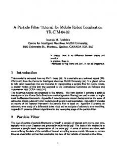
7. Track-Selective Evaluation Framework The empirical proof of track selectivity is achieved by the comparison of localization output and a reference route. This reference must be known in advance and is the true sequence of traveled track IDs. Of special interest is the switch scenario with a splitting switch way run, as shown in Figure 3. Railway switches have a region where the clearance of two vehicles overlap, and only one train can occupy these tracks. There, a false track estimate is tolerated and not a real problem as only one train can occupy the tracks. The length of this tolerance region can either be fixed or individual for every switch, stored within the map. For simplicity reasons, a fixed tolerance of 50 m after a switch start is chosen. The trackselective accuracy is evaluated with the known route (ground truth) and a false track estimate within the tolerance region is marked in orange, a correct estimate is green, and a false one is red. Track precision is defined here as the discrete probability of the track estimate from the filter output. A high precision estimate can be evaluated with an incorrect accuracy, when the true track is different. The track-selective accuracy can be analyzed over time (per second) or over traveled distance (per meter). Train statistics are often related to distance (e.g., millions of train kilometers), so the results are presented in relation to the traveled distance. The method of Algorithm 2 evaluates the train localization estimate of each time step. A cumulative evaluation shows the performance of the localization approach in terms of track selectivity for larger data sets. Each evaluation result is shown relative to the total distance: cum 𝐸error
∑ 𝑒𝑘error = ⋅ 100%, ∑ Δ𝑠𝑘
cum 𝐸switch =
∑ 𝑒𝑘switch ⋅ 100%, ∑ Δ𝑠𝑘
(40)
cum 𝐸OK = 100% − 𝐸switch − 𝐸error .
This method is based on distances which automatically rejects the evaluation of stopped and parked trains. Track-selective errors occur in the presence of parallel tracks. A train run on a route with more single track scenarios will distort an
Algorithm: Track Selective Evaluation Input: Train state 𝑇0:𝑘 , true track IDs 𝐴, map Output: Evaluation: cumulative 𝐸cum , 𝐸cum,𝑝 (1) 𝐵: all track IDs of wrong switch ways from 𝐴, map (2) 𝑃: switch positions from 𝐴, map (3) 𝑙clear. : clearance length of each switch (4) for all train states 𝑇0:𝑘 do (5) 𝑒𝑘switch = 𝑒𝑘error = Δ𝑝𝑘 = 0 (6) if track 𝑖𝑑 is not in 𝐴 (true track ID list) then (7) if 𝑖𝑑 is in 𝐵 & distance to switch < 𝑙clear. then (8) 𝑒𝑘switch = Δ𝑠𝑘 (9) else (10) 𝑒𝑘error = Δ𝑠𝑘 (11) end if (12) end if (13) if other track in the vicinity of 𝑖𝑑𝑘 , 𝑠𝑘 (20 m) then (14) Δ𝑝𝑘 = Δ𝑠𝑘 (15) end if (16) end for (17) compute cumulative evaluation 𝐸cum (40) (18) compute cum. eval. of parallel tracks 𝐸cum,𝑝 (41) (19) return 𝐸cum , 𝐸cum,𝑝 Algorithm 2: Track-selective evaluation over distances.
evaluation in favor of a better track-selective evaluation. An increase of comparability of the evaluation result is considered with a ratio to distances with parallel tracks in vicinity: cum,𝑝 = 𝐸error
cum,𝑝
𝐸switch = cum,𝑝
𝐸OK
∑ 𝑒𝑘error ⋅ 100%, ∑ Δ𝑝𝑘 ∑ 𝑒𝑘switch ⋅ 100%, ∑ Δ𝑝𝑘
(41)
𝑝
𝑝 = 100% − 𝐸switch − 𝐸error .
The switch tolerance evaluation suits mainly for detailed evaluation on small changes and tuning. A compact figure of the evaluation (𝐸) in terms of track selectivity over parallel tracks distances (TS, 𝑃) is the errorfree case of multiple track scenarios: cum,𝑝 . 𝐸TS,𝑃 = 100% − 𝐸error
(42)
This figure explains how good a certain train localization approach performs on a specific track network. This cumulative evaluation is one way to measure the track selectivity performance and contains to some extent the track layout of parallel tracks and switch densities. Another evaluation measure is the error events, which counts and evaluates the transition to the wrong track. One faulty switch resolution results in a cumulative error dependent on the specific track length. A parallel track scenario merges very often by a switch after a station and a wrong output can be on the correct track again. The error event method counts transitions to the error case and respects more the error cause, which is a fault switch way. It differs
Journal of Sensors
11 Table 2: Train routes.
𝐸SW
𝑁 − 𝑁late − 𝑁failed = total ⋅ 100%. 𝑁total
100 80 60 40 20 0
8. Experiment 8.1. Recorded Data Set. The data set was recorded on the regional train “Alstom Coradia Lint 41” under regular passenger service conditions. This train can travel up to 120 km/h and has two drivers’ cabs for two-side operation. Table 2 shows the train runs over 230 km with 107 splitting switches. The train runs on 58.5 km of tracks with other tracks near or in parallel, which are 25.4% of all tracks. The data set contains GNSS PVT data (position, velocity, time) of GPS (Global Positioning System) from a u-blox LEA 6T receiver. The IMU data (Xsens MTi) was recorded with a sample rate of 200 Hz and time stamped from a GPS synchronous clock. For the proposed algorithm, this IMU data was low-pass filtered and downsampled to 4 Hz. The IMU was placed on the front bogie, the GNSS antenna below a fiberglass roof above the bogie position. A special camera (dash-cam) with GPS timestamped video was installed behind the front windshield for the switch way evaluation. 8.2. Labeled Reference Route. The reference for the cross track analysis is a recorded video from the train run. In that video, the motion state can be seen, the switch way and direction of travel. For every run, a reference travel path (i.e., labeled data) can be computed from a start position (GNSS), train direction, the map, and a series of true splitting switch ways. These switch ways are either “left” or “right” and obtained manually from the video.
km 8 8 66 66 8 8 25 25 8 8 230
0
100
200
300 Time (s)
400
500
600
0
100
200
300 Time (s)
400
500
600
(43)
The track-selective evaluation in multiple tracks scenarios 𝐸TS and the switch way resolution evaluation 𝐸SW will be used as compact results.
Time 10 min 10 min 1h 1h 10 min 10 min 30 min 30 min 10 min 10 min 4h
Station (Friedberg)
also in late switch way resolution, if the output is correct again within the correct track which connects to the switch. From these error events, the correct switch way evaluation (𝐸SW ) statistics can be computed of the total split switches 𝑁total , the late resolved switch ways after the switch tolerance 𝑁late and the wrong resolved switch ways 𝑁failed :
Split switches 8 7 22 20 8 7 11 9 8 7 107
Station stop
Forward, backward B F B F B F B F B F 5 × F, 5 × B
Station stop
To station FDB ABG ING ABG FDB ABG AIC ABG FDB ABG
Station (Augsburg)
From station ABG FDB ABG ING ABG FDB ABG AIC ABG FDB
Speed (km/h)
Run 1 2 3 4 5 6 7 8 9 10
Split right Merge Split left
Figure 4: Run 1 over time from Augsburg main station to Friedberg station with known switch ways.
8.3. Implementation. The localization algorithm approaches were implemented within a self-written JAVA framework. This includes the map processing, the sensor data reader, and the evaluation. The sensor data was processed in a causal way; that is, the localization approach processed each measurement in the chronological order and the output was evaluated. No simulated (i.e., generated) data was used. Particle filters are generally computationally expensive by nature. Nevertheless, the temporal performance for (𝑁𝑝 = 100) particles with visualization was processed 19.0 times faster than real time on a laptop (Intel i7M CPU, 2.9 GHz, Windows 7). Hence, a real time operation is possible.
9. Results 9.1. Track Selectivity over Time. Two different evaluations of the reference approach and the proposed algorithm are shown of Run 1 over time. Therefore, the train speed and true switch ways of Run 1 are shown over time in Figure 4. It visualizes the occurrence of splitting switch ways, since their resolution is the challenge for a train localization filter. Figure 5 shows the results of the simple map-matched GNSS positions for Run 1 over time. The correct track is marked with OK in green, an error in the tolerance area in
12
Journal of Sensors Table 3: Detailed cumulative results. OK
Localization (1) Map match GNSS position (2) RBPF, GNSS position (3) Method 2 and GNSS heading (4) Method 2 and IMU yaw rate (5) Method 2 and heading, yaw rate
93.7 (75.2) 94.9 (79.8) 97.3 (89.1) 99.7 (98.9) 99.7 (98.8)
Switch % total distance: 𝐸cum (% parallel tracks: 𝐸cum,𝑝 ) 0.73 (2.86) 1.06 (4.19) 0.26 (1.03) 0.10 (0.41) 0.09 (0.36)
Error
Error events, switch way resolutions 5.57 (21.9) 4.06 (16.0) 2.49 (9.84) 0.17 (0.67) 0.21 (0.84)
108 errors 33 errors 4 switches (1 late, 3 fail) 3 switches (2 late, 1 fail) 4 switches (3 late, 1 fail)
Table 4: Compact track selective results.
Switch tolerance OK
Error
Localization method
0
100
200
300 Time (s)
400
500
600
Figure 5: Track-selective accuracy of simple map-matching (nearest neighbor).
(1) Map match, GNSS pos. (2) RBPF, GNSS pos. (3) (M. 2) + GNSS head (4) (M. 2) + IMU yaw rate (5) (M. 2) + head + yaw rate
Switch way res. Track selectivity (parallel tracks) (107 split switches) 𝐸SW 𝐸TS,𝑃 (58.5 km) 78.1% 84.0% 90.2% 99.3% 99.2%
— 69.2% 96.3% 97.2% 96.3%
Error Switch tolerance OK
0
100
200
300
400
500
600
incorrect track within the tolerance region. The track precision (middle plot) is shortly reduced with the occurrence of split switches as seen in Figure 4. The along precision (bottom plot) is initially coarse but quickly drops after train departure to an average of 1.4 m. This along precision is the weighed empirical deviation of the particle distribution of (37).
Track precision
Time (s) 1 0.8 0.6 0.4 0.2 0
0
100
200
300
400
500
600
700
500
600
700
Along precision (m)
Time (s) 15 10 5 0
0
100
200
300 400 Time (s)
Figure 6: Track-selective accuracy and estimation precision of the Bayesian filter approach: RBPF with GNSS position, heading, and IMU yaw rate.
the vicinity of the switch is yellow, and a wrong track is red. There is no track precision shown, as this approach considers no uncertainty but only the nearest track. Figure 6 shows the accuracy and precision results over time of the realized Bayesian filter with IMU and GNSS of Run 1. At one splitting switch, the filter was estimating an
9.2. Cumulative Track Selectivity. A detailed cumulative evaluation is presented in Table 3. Five localization methods are evaluated, in particular the simple map-matching and four different Rao-Blackwellized particle filter implementations (RBPF). The number of particles is 𝑁𝑝 = 100 in all RBPF evaluations. Each accuracy category is shown in percentage of the total distance of 230 km. As all methods solve the single track scenarios, the track accuracy is shown additionally relative to the total distance of multiple track scenarios (58.5 km) in parenthesis. The evaluation results of a standing train periods are disregarded in this table. The error events in Table 3 indicate how often a transition to wrong tracks happened. Depending on the method, this can be traced back to faulty switch resolution. A late switch error represents a resolved switch way after the evaluation threshold, whereas a failed switch relates to a wrong resolved switch way. The compact results according to (42) and (43) are presented in Table 4. There are no switch way resolution results for Method 1 as the simple map-match considers only the nearest track and does not resolve a switch way.
10. Discussion 10.1. Discussion on Results. One major goal of train localization is a track-selective estimation result. As seen from
Journal of Sensors Table 3, Method 1 (reference approach of simple mapmatching) has severe problems to determine the correct track at 21.9% of parallel tracks. The proposed algorithm RBPF uses also GNSS positions (Method 2) but shows some improvement with 16.0% of wrong tracks on multiple track scenarios for 33 times. The filtered methods, especially the last three, converge to one track in a parallel track scenario. There, the switch resolution is essential and a failed switch forces the estimate to stay on the wrong track until a merging switch to the true track corrects the estimate again. For example, Method 3 shows an improvement in error events but stays three times on a wrong, parallel track. The best results are achieved with Method 4 (RBPF with yaw rate) on 99.3% of parallel tracks which relates to an error of 6.7⋅10−3 and stands for a false localization on 394 m (24.8 s) in total. With two late and one failed resolved switch way, Method 4 achieves 97.2% in switch way resolution, respective of an error of 2.8 ⋅ 10−2 . The definition or adjustment on the switch way evaluation threshold has direct impact on the results and was 50 m. In case this threshold tends to 0 m, the track-selective results over distance can be extracted from the “OK” column of Table 3 and are slightly worse. However, the switch way resolution results of (43) will severely decrease with a zero tolerance area by many late resolved switches. The results are quite sensitive to the parameters such as measurement noise, the noise ratio of different measurements, resampling occurrence, process, and sampling noise as well as the map quality. Better or even perfect results may be expected by exhaustive optimization of the map and filter parameters. As an unwanted consequence, map and parameters may match this limited data set and the results loose generality. Nevertheless, the following tendencies can be seen from the results: the additional use of the GNSS heading (Method 3) shows only little improvements with 9.8% in terms of errors compared to Method 2 (GNSS position only). Further, the combination of all likelihoods of Method 5 (GNSS position and heading, IMU yaw rate) does not show an improvement. The most likely explanation of this effect might be the map with its coarse heading and curvature geometry. These values are derived from positions and are consequently dependent. Slightly wrong positions cause an error in both values. Because of this dependency the combination of the measurements has no further gain in accuracy. For the realized implementation of the sequential Bayesian filter, the particle filter approach was chosen, as the particles can sample the different hypotheses and any nonlinear distribution. The Rao-Blackwellization marginalizes the linear state variables and estimates them with a Kalman filter. As a consequence, the particle filter samples only the cross track hypotheses (𝑖𝑑) and the along positions (𝑠). The number of particles are relatively low (𝑁𝑝 = 100) as the particles are limited and constraint on the tracks. Additionally, the linear state variables are estimated by nested Kalman filters (RaoBlackwellization). A particle filter approximates distributions and induces two times additional noise as a tradeoff for convergence reasons: the sampling adds noise, which is
13 needed to maintain particle diversity as well as the resampling in order to avoid particle depletion and divergence. 10.2. Comparison. Lauer and Stein [13] (GNSS, velocity sensor) showed a gain in confidence about the track decision between a simple map-match and the proposed estimation algorithm. A similar gain can be seen between simple mapmatch (Method 1) and RBPF with GNSS positions only (Method 2). B¨ohringer [6] received slightly better trackselective results (99.78%) compared to Method 4 (99.33%) with a different data set and an algorithm with additional eddy current sensor as switch way detector. Hensel et al. [12] do not consider explicit figures on switch way resolution. From switch detection and classification rates over 99%, a switch way resolution may be deduced with a similar performance. In comparison, Method 4 reaches 97.2% of correct switch way resolution even without an eddy current sensor and a coarse geometric map from OSM data. However, a direct comparison between other approaches is not obvious as different data sets and different evaluation metrics are in use. Therefore, comparative results can be seen as quite similar as the differences are marginal for different data sets and metrics. Finally, from the literature and the present results, it can be reasoned that most of the gain in accuracy can be achieved by using an estimation filter as well as using sensors which can measure the competing switch ways. As this is quite expectable, further investigations are necessary to identify the smaller gains and differences of varied filters or sensor fusion approaches on the same data set.
11. Proposed Enhancements Several directions of performance improvements of train localization are identified. 11.1. Advances of the RBPF. The particle filter can be improved with advanced procedures for better particle diversity on along track. Secondly, an enhanced resampling timing may be investigated, which suspends resampling near switches for an undisturbed switch way resolution. 11.2. Improved Odometry. The along-track odometry can be extended with slope estimation from IMU pitch rate integration, map information about slope, or gravity vector estimation from acceleration measurements. A slope consideration would increase the accuracy of relative alongtrack estimation and also increase the range to propagate localization in GNSS denied areas. 11.3. Additional Sensors. A further increase in track-selective accuracy, outage robustness, and redundancy can be considered with the use of extrinsic sensors, such as magnetic sensors, cameras, LIDAR, or aperture radar with direct switch way measurements. 11.4. More Accurate Map. An accurate curvature and heading information in the map is a crucial factor for a correct switch
14 way resolution with GNSS and IMU. The major advantage of generating a map from an OSM data base is to obtain a track map of a certain railway network size with a sufficient number of tracks. A map generation approach from onboard sensor data is presented in [7, 21]. Furthermore, a direct comparison of alternative methods and sensors may be evaluated with same data sets and evaluation metrics. Studies could investigate the accuracy of different algorithms (e.g., multihypothesis filter versus particle filter), or the accuracy gain of different sensor data integration schemes (e.g., loosely coupled GNSS versus tightly coupled).
12. Summary This paper presents a probabilistic train localization approach with a track-selective evaluation. In contrast to other approaches, this train localization comprises a Rao-Blackwellized particle filter (RBPF), a map of the railway tracks and sensor data of a GNSS receiver (Global Navigation Satellite System), and an IMU (inertial measurement unit). A novel RBPF implementation is presented which estimates the train localization posterior recursively. The Rao-Blackwellization marginalizes the linear state variables and estimates them with a Kalman filter. As a consequence, the particle filter samples only the cross track hypotheses (𝑖𝑑) and the along positions (𝑠). The RBPF estimates directly the topological track coordinates; that is, the particles stay on the tracks. Further, a particle distribution can handle different track hypotheses and other nonlinear distributions. The map contains prior knowledge for the measurement models such as the track geometry data. The RBPF is able to resolve the unknown train-to-track orientation at initialization and can handle forward and backward runs of the train. A novel evaluation method for track selectivity evaluates the localization results with real data recorded from a regional train. This generic evaluation method can be used to generate more comparable results of different approaches with different sensors and measurement data. Train runs were analyzed over 230 km of tracks with 107 split switches and parallel track scenarios of 58.5 km. Further improvements for a safety-of-life train localization of the special realization are discussed towards higher reliability of track selectivity. The best combination of RBPF filter with GNSS positions and IMU yaw rates showed a track-selective performance of 99.3% on tracks with multiple tracks in the vicinity and 97.2% of successfully resolved switch ways within the tolerance. The realized RBPF approach with GNSS, IMU, and a track map showed promising results towards a track-selective and continuous train localization even with low-cost sensors and runs in real time.
Competing Interests The author declares that there are no competing interests.
Journal of Sensors
Acknowledgments The author wants to thank the railway transportation company BRB (“Bayerische Regiobahn”) for the support with the measurements, Andreas Lehner (DLR) for the map, Omar Garcia Crespillo (DLR) for initial software implementations, Stephan Sand (DLR) for proofreading, and Christoph G¨unther (DLR) for comments.
References [1] T. Strang, M. Meyer zu Hoerste, and X. Gu, “A railway collision avoidance system exploiting ad-hoc inter-vehicle communications and galileo,” in Proceedings of the 13th World Congress and Exhibition on Intelligent Transportation Systems and Services (ITS ’06), London, UK, October 2006. [2] T. Strang, Railway Collision Avoidance System, 2015, http://www .collision-avoidance.org. [3] O. Heirich, P. Robertson, A. C. Garc´ıa, T. Strang, and A. Lehner, “Probabilistic localization method for trains,” in Proceedings of the Intelligent Vehicles Symposium (IV ’12), pp. 482–487, IEEE, Alcal´a de Henares, Spain, June 2012. [4] O. Heirich, P. Robertson, A. Cardalda Garcia, and T. Strang, “Bayesian train localization method extended by 3D geometric railway track observations from inertial sensors,” in Proceedings of the15th International Conference on Information Fusion (FUSION ’12), pp. 416–423, Singapore, July 2012. [5] O. G. Crespillo, O. Heirich, and A. Lehner, “Bayesian GNSS/IMU tight integration for precise railway navigation on track map,” in 2014 IEEE/ION Position, Location and Navigation Symposium, PLANS 2014, pp. 999–1007, usa, May 2014. [6] F. B¨ohringer, Gleisselektive ortung von schienenfahrzeugen mit bordautonomer sensorik [Ph.D. dissertation], Universit¨at Karlsruhe (TH), Karlsruhe, Germany, 2008. [7] C. Hasberg, S. Hensel, and C. Stiller, “Simultaneous localization and mapping for path-constrained motion,” IEEE Transactions on Intelligent Transportation Systems, vol. 13, no. 2, pp. 541–552, 2012. [8] O. Plan, GIS-gest¨utzte verfolgung von lokomotiven im werkbahnverkehr [Ph.D. dissertation], University of German Federal Armed Forces, Munich, Germany, 2003. [9] K. Gerlach and C. Rahmig, “Multi-hypothesis based mapmatching algorithm for precise train positioning,” in Procedings of the 12th International Conference on Information Fusion (FUSION ’09), pp. 1363–1369, Seattle, Wash, USA, July 2009. [10] A. Broquetas, A. Comer´on, A. Gelonch et al., “Track detection in railway sidings based on MEMS gyroscope sensors,” Sensors, vol. 12, no. 12, pp. 16228–16249, 2012. [11] O. Heirich, A. Lehner, P. Robertson, and T. Strang, “Measurement and analysis of train motion and railway track characteristics with inertial sensors,” in Proceedings of the 14th International IEEE Conference on Intelligent Transportation Systems (ITSC ’11), pp. 1995–2000, IEEE, Washington, DC, USA, October 2011. [12] S. Hensel, C. Hasberg, and C. Stiller, “Probabilistic rail vehicle localization with eddy current sensors in topological maps,” IEEE Transactions on Intelligent Transportation Systems, vol. 12, no. 4, pp. 1525–1536, 2011. [13] M. Lauer and D. Stein, “A train localization algorithm for train protection systems of the future,” IEEE Transactions on Intelligent Transportation Systems, vol. 16, no. 2, pp. 970–979, 2015.
Journal of Sensors [14] J. Wohlfeil, “Vision based rail track and switch recognition for self-localization of trains in a rail network,” in Proceedings of the IEEE Intelligent Vehicles Symposium (IV ’11), pp. 1025–1030, IEEE, Baden-Baden, Germany, June 2011. [15] R. Ross, “Track and turnout detection in video-signals using probabilistic spline curves,” in Proceedings of the 15th International IEEE Conference on Intelligent Transportation Systems (ITSC ’12), pp. 294–299, Anchorage, Alaska, USA, September 2012. [16] D. Stein, M. Lauer, and M. Spindler, “An analysis of different sensors for turnout detection for train-borne localization systems,” in Computers in Railways XIV, vol. 135 of WIT Transactions on The Built Environment, WIT Press, 2014. [17] C. Rahmig, L. Johannes, and K. L¨uddecke, “Detecting track events with a laser scanner for using within a modified multihypothesis based mapmatching algorithm for train positioning,” in Proceedings of the European Navigation Conference (ENC ’13), Vienna, Austria, April 2013. [18] C. Fouque and P. Bonnifait, “Matching raw GPS measurements on a navigable map without computing a global position,” IEEE Transactions on Intelligent Transportation Systems, vol. 13, no. 2, pp. 887–898, 2012. [19] S. S. Saab, “A map matching approach for train positioning. I. Development and analysis,” IEEE Transactions on Vehicular Technology, vol. 49, no. 2, pp. 467–475, 2000. [20] F. Gustafsson, F. Gunnarsson, N. Bergman et al., “Particle filters for positioning, navigation, and tracking,” IEEE Transactions on Signal Processing, vol. 50, no. 2, pp. 425–437, 2002. [21] O. Heirich, P. Robertson, and T. Strang, “RailSLAM— localization of rail vehicles and mapping of geometric railway tracks,” in Proceedings of the IEEE International Conference on Robotics and Automation (ICRA ’13), pp. 5212–5219, IEEE, Karlsruhe, Germany, May 2013. [22] Open Street Map (OSM), 2015, http://www.openstreetmap.org. [23] P. Misra and P. Enge, Global Positioning System: Signals, Measurements, and Performance, Ganga-Jamuna Press, Lincoln, Mass, USA, 2006. [24] A. Doucet, N. De Freitas, K. Murphy, and S. Russell, “Raoblackwellised particle filtering for dynamic bayesian networks,” in Proceedings of the 16th Conference on Uncertainty in Artificial Intelligence, Morgan Kaufmann Publishers, Stanford, Calif, USA, June-July 2000. [25] F. Gustafsson, Statistical Sensor Fusion, Studentlitteratur, Lund, Sweden, 2012. [26] M. S. Arulampalam, S. Maskell, N. Gordon, and T. Clapp, “A tutorial on particle filters for online nonlinear/non-Gaussian Bayesian tracking,” IEEE Transactions on Signal Processing, vol. 50, no. 2, pp. 174–188, 2002. [27] F. Daum and J. Huang, “Curse of dimensionality and particle filters,” in Proceedings of the IEEE Aerospace Conference, pp. 1979–1993, March 2003.
15
International Journal of
Rotating Machinery
Engineering Journal of
Hindawi Publishing Corporation http://www.hindawi.com
Volume 2014
The Scientific World Journal Hindawi Publishing Corporation http://www.hindawi.com
Volume 2014
International Journal of
Distributed Sensor Networks
Journal of
Sensors Hindawi Publishing Corporation http://www.hindawi.com
Volume 2014
Hindawi Publishing Corporation http://www.hindawi.com
Volume 2014
Hindawi Publishing Corporation http://www.hindawi.com
Volume 2014
Journal of
Control Science and Engineering
Advances in
Civil Engineering Hindawi Publishing Corporation http://www.hindawi.com
Hindawi Publishing Corporation http://www.hindawi.com
Volume 2014
Volume 2014
Submit your manuscripts at http://www.hindawi.com Journal of
Journal of
Electrical and Computer Engineering
Robotics Hindawi Publishing Corporation http://www.hindawi.com
Hindawi Publishing Corporation http://www.hindawi.com
Volume 2014
Volume 2014
VLSI Design Advances in OptoElectronics
International Journal of
Navigation and Observation Hindawi Publishing Corporation http://www.hindawi.com
Volume 2014
Hindawi Publishing Corporation http://www.hindawi.com
Hindawi Publishing Corporation http://www.hindawi.com
Chemical Engineering Hindawi Publishing Corporation http://www.hindawi.com
Volume 2014
Volume 2014
Active and Passive Electronic Components
Antennas and Propagation Hindawi Publishing Corporation http://www.hindawi.com
Aerospace Engineering
Hindawi Publishing Corporation http://www.hindawi.com
Volume 2014
Hindawi Publishing Corporation http://www.hindawi.com
Volume 2014
Volume 2014
International Journal of
International Journal of
International Journal of
Modelling & Simulation in Engineering
Volume 2014
Hindawi Publishing Corporation http://www.hindawi.com
Volume 2014
Shock and Vibration Hindawi Publishing Corporation http://www.hindawi.com
Volume 2014
Advances in
Acoustics and Vibration Hindawi Publishing Corporation http://www.hindawi.com
Volume 2014