functions, which is also referred to as the partition-of-unity method. The reconstruction ..... Loopy BP [26] can be applied to obtain good approximation results. 3.3. .... the loop of Algorithm 2 to invoke a direct solution routine when the iteration ...
A Partition-of-Unity Based Algorithm for Implicit Surface Reconstruction Using Belief Propagation Yi-Ling Chen Shang-Hong Lai∗ Department of Computer Science National Tsing Hua University, Hsinchu, Taiwan Abstract In this paper, we propose a new algorithm for the fundamental problem of reconstructing surfaces from a large set of unorganized 3D data points. The local shapes of the surface are recovered by variational implicit surface represented as a weighted combination of radial basis functions. The variational implicit patches are then combined together to form the overall surface via a set of blending functions, which is also referred to as the partition-of-unity method. The reconstruction algorithm first partitions the input point set by octree subdivision and surface normal estimation is performed so as to orientate the local variational implicit patches. A new graph optimization scheme based on the belief propagation framework is proposed to determine the global consistent orientation for the entire set of data points. To achieve multi-scale reconstruction, we propose a novel progressive reconstruction algorithm which utilizes the Schur complement formula to reduce the computational cost of iteratively updating the radial basis function coefficients. Finally, we demonstrate the performance of the proposed algorithm by showing experimental results on some real-world 3D data sets.
1. Introduction The shape of a 3D object is usually represented as a 3D point cloud. The acquisition of sample points may be from a diversity of sources, such as range scanners or stereo vision systems. However, the point cloud alone only conveys partial information of an object and does not provide a complete description of the surface. A more suitable surface representation is needed for the purpose of further processing, e.g. texture mapping, visualization or rendering applications. Therefore, a number of algorithms [1, 2, 7, 8, 11, 14] have been developed to reconstruct a “full” surface model, such as polygonal meshes, from a set of discrete samples on the objects. This problem of surface reconstruction, which is to recover a digital 3D model ∗ {yilin,lai}@cs.nthu.edu.tw
Figure 1. The proposed algorithm is capable of reconstructing fine-quality implicit surfaces from an unorganized point cloud efficiently (left). A multi-scale representation enables us to control the level of detail by evaluating the implicit function at the desired resolution (right).
from a set of 3D data points for an existing physical object, is ill-posed because much information might be lost during the data acquisition process, thus it has been an important research topic in the fields such as, computer graphics, computer vision, scientific visualization, computer-aided design (CAD) and medical imaging. For the need of a general surface reconstruction algorithm, we consider the fundamental problem of surface reconstruction from a large unorganized 3D data set with no additional information, such as surface normal or topology, assumed to be known in advance. The reconstruction algorithm should be able to infer all necessary information automatically and generate a piecewise smooth surface as output. In essence, our method could be regarded as an extension of two well-known techniques. Firstly, the unknown surface is subdivided into local shape functions and later smoothly blended together through a set of blending
functions, which is known as the partition-of-unity (POU) method introduced by Ohtake et al. [14]. In addition, for the choice of the underlying surface representation, we apply the variational technique developed by Turk et al. [23] to find the local interpolation implicit function which is defined as a linear combination of radial basis functions. In our approach, the input sample points are firstly subdivided by an octree and local tangent planes are fitted at each point to estimate its normal vector in order to orientate the local variational patches. As the problem described by Hoppe et al. [11], the main challenge facing the algorithm is the selection of the normal directions so as to define the globally consistent orientation for the entire data set. Instead of using their orientation propagation method based on traversing a minimal spanning tree constructed over the surface model, we propose to determine the globally consistent orientation by propagating beliefs over local Riemannian graphs with the surface sample points treated as its nodes. The inside/outside test is performed by applying the well-known Belief Propagation algorithm to infer the maximum a posteriori (MAP) solution of the label of the surface normal vectors. The creation of variational implicit surfaces is sometimes criticized for its high time complexity. Moreover, due to the global support of the basis functions, it requires repetitive computation of RBF coefficients to progressively reconstruct implicit surfaces in a coarse-to-fine fashion. In this paper, we propose a novel algebraic approach based on the Schur complement formula to simplify the computation involved in the progressive reconstruction. The main contributions of this work can be summarized as follows: • We propose an efficient 3D surface reconstruction algorithm based on the variational implicit surface representation in the partition-of-unity framework. It is very efficient in both time and memory storage; • A novel graph optimization formulation is proposed for robust estimation of the globally consistent orientation for the entire data set. The graph optimization is accomplished by using the Belief Propagation algorithm to develop an efficient algorithm; • A new iterative greedy algorithm utilizing the Schur complement formula is proposed to efficiently update the RBF coefficients for progressive implicit surface reconstruction.
2. Background and Related Works 2.1. Implicit Surfaces Generally speaking, in spite of the diversity of the underlying mathematical forms, implicit surfaces typically aim to find a scalar-valued continuous function f , whose zero
level-set describes the unknown surface. The implicit function f partitions the space into two parts: inside and outside of the surface, where it takes positive and negative values, respectively. Compared to explicit surface models, implicit surface modeling possesses the advantages of being robust to noises and non-uniform sampling density, and easy to convert into other representations and perform CSG operations. The pioneering works on implicit surfaces include the blobby surface [3] that are sum of implicit primitives such as Gaussian blobs. Hoppe et al. [11] introduced the concept of modeling surface as a signed distance field which is defined as the distance to locally fitted tangent planes. Curless and Levoy [7] proposed an efficient algorithm to integrate a set of range scans to build the signed distance function. Another important class of implicit modeling is based on the variational formulation for surface reconstruction, which leads to the implicit surface solution represented as a radial basis function (RBF). Its recent development will be discussed in the next section. A thorough description of the wide variety of implicit surfaces is obviously beyond the scope of this paper. More detailed introduction to implicit surfaces can be found in the book by Bloomenthal et al. [5].
2.2. Variational Method and RBFs The notion of interpolating implicit surfaces was firstly introduced by Savchenko et al. [19], later developed by Turk et al. [23] for shape transformation, and applied to a variety of applications successfully [9, 10]. Interpolating implicit surface attempts to find a smooth embedding function f : �d → � that exactly passes the specified locations by using mathematical tools from variational calculus. Therefore, this class of implicit surface is also known as variational implicit surface. In a nutshell, the variational method imposes an additional smoothness constraint that minimizes the aggregate curvature of the function, thus leading to the smoothest function among all possible solution functions satisfying the interpolation conditions. The variational approach is a general solution to the d-dimensional scattered data interpolation problem. Consider the following problem: given a set of N constraint points C = {c1 , c2 , . . . , cN } that are scattered on or near the unknown surface with the corresponding scalar fields h1 , h2 , . . . , hN . Find f that satisfies the interpolation conditions: f (ci ) = hi , i = 1, 2, . . . , N. To solve the aforementioned energy minimization problem, the interpolation function f is expressed in terms of a weighted combination of radial basis functions, which can be written as follows:
f (x) =
N �
wj φ(x − cj ) + P (x),
(1)
j=1
where cj = (xj , yj , zj ) are the locations of the constraints, wj are the weights, and P (x) is a degree one polynomial accounting for the linear and constant term of f . There is a rich variety of radial basis functions suggested in the literature. For 3D interpolation, we adopt the pseudo-cubic basis function φ(r) = r3 , as also used in [23]. Solving for the unknowns, wj , and the coefficients of P (x) involves forming a linear system given below: �� � � � � A P w h = (2) λ 0 PT O where Aij = φ(�ci − cj �). The polynomial part of the interpolation function f in (1) has the form of P (x) = λ0 + λ1 x + λ2 y + λ3 z, and thus P is the matrix with the i-th row being (1, xi , yi , zi ). Note that the sub-matrix A in (2) is positive-definite and a closed-form solution always exists under very mild conditions. However, because RBFs are globally supported in nature, the linear system in question is also dense and its size grows exponentially with respect to the number of constraints, making it computationally intractable to solve by direct methods, such as LU decomposition or SVD, because their computational complexity is O(N 3 ). To alleviate the problem of high computational cost, Carr et al. [6] applied the far field expansion method for fast fitting and evaluation of variational interpolant of numerous basis functions. However, the drawback of their method is that the far field expansion method is difficult to implement. By cooperating with the partition-ofunity method described in the next section, the complexity of variational implicit surface can be well controlled and easily extended to handle with large models. Another issue regarding variational interpolation is the specification of non-zero valued constraints. Non-zero valued constraints not only avoid trivial solution (in the case that all the scalar fields equal to zero) but also provide guidance for f to indicate the interior and exterior region of the space. One commonly used strategy for creating such constraints is to project constraint points along their normal directions [24, 23, 6, 10]. For more details about constraint specification, the interested readers are referred to the original paper by Turk et al. [24].
2.3. Partition-of-Unity Framework The partition-of-unity method has attracted much attention in recent research of implicit surface modeling. The concept behind it can be traced back to Shepard’s blending method [20], which was originally designed to build a global function by subdividing the problem domain into a set of sub-domains where locally defined functions are
solved and provides a good means of smoothly blending the local solution functions to form a good approximation for the global solution of interest. With ωi denoted as the set of non-negative and compactly supported weighting functions assigned to the local functions fi , the blended function f can be expressed as below: � i ωi (x)fi (x) , (3) f (x) = � i ωi (x) Based on this framework, many hierarchical reconstruction algorithms have been proposed. The Multi-level Partition-of-Unity (MPU) implicits method introduced by Ohtake et al. [14] used an octree-based adaptive approach for surface reconstruction from a large and accurate data set. Sharp features can be well preserved by local selection of fitting models. Xie et al. later extended the MPU implicit to handle noisy data sets [28]. They employed an active contour method and a voting process for orientation determination. Tobor et al. [22] proposed a multi-scale reconstruction algorithm by building a binary tree decomposition and performing a bottom-up thinning operation.
3. Global Consistent Orientation Inference 3.1. Overview As discussed in Section 2, the implicit surface consists of many local variational interpolants, which are blended as a pseudo-signed distance field through the partition-ofunity method. To correctly blend the local shape functions, they should have been properly and consistently oriented in advance. In our approach, the input data set is firstly subdivided by an octree for further local shape recovery and the normal directions are estimated by fitting a local tangent plane to each data point and its neighborhood [17, 11]. Given the normal vector ni of each point ci , we are uncertain of which part of the model it is directed to, say, inside or outside. The goal of global consistent orientation inference is to determine for each point, ci , a label xi such that all the normal vectors are consistently aligned to be directed to either interior or exterior regions subject to the model. The overall optimization is formulated as solving a graph labeling problem. The algorithm proceeds by iteratively constructing a local graph and applying a belief propagation algorithm to find a label xi ∈ {0, 1}, which corresponds to exterior and interior regions of the model, respectively. Analogous to other orientation alignment schemes [11, 29], the global consistent orientation is obtained by flipping the normal vectors with labels different from that of a pre-selected seed point.
3.2. Belief Propagation Optimization In detail, let us reconsider the problem by starting from a set of 3D data points that are geometrically close to each
other. We construct a Riemannian graph G = {V, E} with each node in V corresponding to one of the 3D points. Specifically, a Riemannian graph G is defined as an undirected graph among which there exists an edge eij in E if vj is one of the k-nearest-neighbor of vi , and vice versa. We define the following energy on G: � � Ed (xi ) + Es (xi , xj ), (4) E(X ) = (i,j)∈E
i∈V
where Ed (xi ) = xi , Es (xi , xj ) = −1(xi +xj ) · αij , Note that Ed (xi ) is the data energy measuring how well the estimated labels fits to our prior knowledge about the model. Here we set Ed to be just the label of node i, and it acts as an additional constraint that selects two of the optimal label sets X with more nodes labeled as zero. Intuitively, the consistency of two normal vectors can be defined as their inner product, which is positive if they have consistent orientations and negative otherwise. By letting αij be −ni · nj , Es (xi , xj ) behaves like a smoothness energy which penalizes the inconsistent changes of normal orientations associated with two neighboring nodes. The optimal labels for all nodes are obtained by minimizing the total energy E(X ). In a sense, the graph G can be thought of as a joint probability of a set of binary random variables with the edges indicating the dependency between distinct nodes. The inference of marginal probability of a specific node means that we have to sum over all the possible states of other nodes, which can be a very laborious process. Belief Propagation (BP) is an efficient probability inference algorithm proposed by Pearl [18], which has recently been proven to be very effective in many computer vision and image processing problems [21, 25]. It comes with two variants: sumproduct and max-product. In this paper, we use the maxproduct algorithm to find a MAP solution formulated earlier in this section by taking negative log probabilities. Briefly speaking, Belief Propagation works by iteratively propagating messages or beliefs along edges over a graph. Let us denote the message sent from node i to j as mi→j . In our formulation, message mi→j is a two-dimensional vector, and can be regarded as the probability density function that node j takes label of 0 or 1. The local message passing mechanism is for each node to receive and update message by forming product of incoming messages and local evidence as the following equation: mi→j (xj ) = Z max(Ed (xi ) · Es (xi , xj )· xj
� u∈N bhd(i)\j
mu→i (xi )),
(5)
Figure 2. Starting from a seed cell, the advancingfront algorithm traverses the unchecked data points of the model to perform orientation inference.
where N bhd(i)\j denotes the neighbors of i other than j, and Z is a normalization factor. Finally, the MAP solution for each node i is computed as x∗i = Z max(Ed (xi ) · xi
�
mu→i (xi )),
(6)
u∈N bhd(i)
For tree structured graphs, BP is guaranteed to converge to a fixed message m∗ after at most T iterations depending on the longest path of the graph. For graphs with loops, Loopy BP [26] can be applied to obtain good approximation results.
3.3. Advancing-Front Algorithm Intuitively, to obtain the optimal label of each data point, a graph consisting of all the data points should be constructed for the energy minimization procedure. However, we choose to infer the normal orientation locally and iteratively propagate the orientation to obtain the global solution due to the following two observations: 1. The interaction between normal orientations is essentially a local property. As a result, local orientation inference typically gives accurate results. That is the reason that we construct a Riemannian graph that only encodes the information of proximity. 2. Previous results provide additional information for further inference.
Algorithm 1 OrientationPropagate(F = null) Seed selection. Find cell v containing the seed point, insert v into F . while F not empty do active cell v = F .front; collect node set V; construct Riemannian graph G with V; perform BP on G; update labels of V; find and insert adjacent non-empty cells of v into F ; end while return
Therefore, we devise the following advancing-front algorithm: Initially, we have the position of each point associated with its normal vector unaligned. Starting from a seed point with its normal orientation as the basis for alignment. Echoing the octree subdivision process, the approach proceeds by iteratively marching an active cell or voxel to traverse the unchecked data points until all the data points have been checked. We adopt the seed selection procedure as described in [11]. Our algorithm maintains a data structure of front F , which contains a queue of candidate cells to be selected for orientation inference process in the next iteration. The basic idea of the incremental algorithm is straightforward: traversing all the non-empty leaves among the octree in the order of connected components of visited cells. The belief propagation inference is performed on a graph constructed subject to the active cell. The sixth line of Algorithm 1 involves a process of collecting points within the active cell as the set of nodes for graph construction. The process also searches adjacent cells for points whose orientations have been determined in previous iterations to provide evidence for orientation inference. The main concern is the depth of octree, which depends on the feature size. It is important to prevent the size of cell from being too large such that unconnected components of the modeled surface will be included in a cell. To keep the graph remaining a manifold avoids mistakenly aligning the orientation of an independent part of the model to another, such as two opposite sheets close to each other. The depth of the octree is determined by a user-specified parameter because Algorithm 1 is not currently an adaptive algorithm.
4. Progressive Reconstruction 4.1. Schur Complement Formula To establish a progressive or multi-scale of implicit surfaces is attractive especially with extremely large and complex models. are expensive to store, transmit and render.
representation when dealing Such models A multi-scale
Figure 3. Reconstructed implicit surfaces by using direct RBF updating (left) and Schur complement updating (right).
implicit surface can be used to compress or simplify the surface representation by using the most significant data points only. A coarse surface can be refined by adding additional data points. However, because of the global support nature of radial basis functions, adding only a few new data points leads to complete re-computation of the resulting RBF coefficients. In [13], Morse et al. used basis functions with compact support to speed up the process of creating implicit surfaces by solving a sparse matrix. Although using compactly supported RBFs [27] leads to more efficient computation in determining the RBF coefficients, it has the drawback that holes or irregular sampled regions may not be interpolated or repaired well. In [15], Ohtake et al. introduced a multilevel interpolation approach that combines quadrics multiplied by compactly supported radial weights and offsetting functions. In this paper, we propose an algebraic approach to alleviate the cost of iteratively updating globally supported radial weights by using the Schur complement formula [16]. Schur complement formula gives the closed-form expression for the inverse of a partitioned matrix. Firstly, we rearrange the linear system in equation (2) as below: �� � � � � λ 0 O PT = (7) h w P A The matrix of our progressive reconstruction problem can thus be expressed by the following 2 × 2 partitioned matrix: � � K11 K12 K= (8) K21 K22 where K11 is simply the linear system of (7) formed by T conthe existing RBF centers. The sub-matrix K12 = K21 tains the interaction between the newly added centers and existing centers. K22 is a square matrix corresponding to the newly added centers. To update the old coefficients and
solve for the new ones, we need to solve the linear system Kw = h. According to Schur complement formula, the inverse matrix K −1 can be written in the following form: K −1 = where
�
−1 −1 −1 K11 + K11 K12 S −1 K21 K11 −1 −1 −S K21 K11
−1 −K11 K12 S −1 S −1 (9)
−1 K12 S = K22 − K21 K11
Compared with solving the overall linear system with O(N 3 ) techniques, e.g. LU decomposition or SVD, we can see that the computation of K −1 involves only multiplication of the partitioned matrices, which has lower cost. Note −1 , which is the inverse matrix corresponding to the that K11 −1 , old RBF coefficients, is extensively used. By storing K11 we can exploit the Schur complement formula to solve the new linear system with low cost.
4.2. Partition-of-unity Implicits Algorithm 2 buildPOU(cell, ε, δ) if fi is not created yet then Select initial RBF center set C0 and create fi ; Evaluate the residual rj at each data point cj ; end if while max(|rj |) > ε and size(Ci ) < δ do Append new centers with largest residuals to form Ci+1 ; Re-compute fi by equation (9); Refresh residual ri ; end while if max(|rj |) > ε then for each cell→child, invoke buildPOU(child, ε, δ); end if return With the matrix machinery introduced in the previous section, we are able to devise a simple greedy algorithm to iteratively refine the local implicit fi to meet the desired fitting accuracy ε. Initially, only a coarse set of data points C0 are selected as RBF centers to compute fi . We evaluate fi to calculate the residuals at each unused data points, which will be used as the stopping criterion. If the maximum residual is less than the specified accuracy ε, the iterative refinement procedure is stopped. Otherwise, the data points with largest residuals are appended to form a new list Ci of RBF centers and the coefficients are updated by applying the Schur complement formula. Combined with the partition-of-unity framework, we recursively partition the region of space occupied by the input set of data points, and apply the above procedure to build the local RBF approximations. Our formulation is similar with the octree-based
Table 1. Performance of the proposed algorithm. Computation times are represented in seconds.
�
N
level
BP
RBF
Bunny
35647
5
31.44
8.12
Santa
75781
5
67.89
4.53
Igea
134345
6
124.38
41.76
Armadillo
172970
6
163.42
46.82
algorithm proposed by Ohtake et al. [14]. The main difference is the iterative refinement procedure. Because of the exact interpolation property of variational implicit surfaces, the algorithm attempts to enhance the accuracy of local shape functions by using more RBF centers before the subdivision. To prevent the local shape functions from growing too large, we regularly examine if the size of Ci is larger than a pre-defined threshold δ. If the size of Ci exceeds δ, we resort to subdivision for the purpose of better approximation as well as complexity control. In practice, for real-world models with large amount of data points, it is difficult to model the surface with only a few local functions. Therefore, it is advantageous to start from an appropriate level of the octree to skip the intermediate process. The pseudo-code listed in Algorithm 2 illustrates the recursive construction procedure of our algorithm. One drawback of the progressive RBF coefficient update by using Schur complement formula is that it introduces accumulated numerical errors during each iteration. The numerical errors can be eliminated by solving the inverse matrix directly. This can be achieved by setting a sentinel counter in the loop of Algorithm 2 to invoke a direct solution routine when the iteration count gets large and the errors become noticeable. In our implementation, we empirically set the guarding variable to 10 for all the experiments.
5. Experimental Results All of the examples presented in the paper are generated on a standard PC with Pentium 4 3.4 GHz CPU and 1 GB RAM. In addition, we use Bloomenthal’s implicit surface polygonizer [4] to extract a triangular mesh of the reconstructed implicit surface for visualization. Many of the subproblems discussed above require extensive searching for the nearest neighbors of a specific data point, such as local tangent plane fitting and Riemannian graph construction. We apply a spatial partitioning technique, say, k-D tree for solving the range searching problem more efficiently. The input data set is scaled and inserted into a unit bounding cube. Then, an octree-based hierarchy is constructed and local variational implicits are computed
and refined until a desired accuracy is achieved. We use a B-spline based weighting function as suggested in [14] for partition-of-unity blending. The blended function can be evaluated at different levels for multi-scale reconstruction. Fig. 4 illustrates the capability of the proposed algorithm to reconstruct implicit surfaces from real-world data sets accurately and efficiently. Fig. 5 illustrates an example of coarse-to-fine reconstruction. Table 1 summarizes the computation time of several models evaluated at different octree levels. We set the fitting accuracy to 5 × 10⁻⁴ for all cases. The orientation propagation timings are also included.
6. Conclusions and Future Directions In this paper, we presented a novel approach to reconstruct implicit surface from unorganized points by employing the partition-of-unity method and variational technique. To determine the global consistent oientation of the model being recovered, we apply the belief propagation algorithm to perform local orientation inference and iteratively advance the current inference result in a front-propagation fashion. According to our experiment, the proposed orientation inference algorithm can correctly align the normal vectors to be orientated consistently. In addition, a novel scheme is proposed to progressively refine the local variational shape functions. The greedy iterative refinement procedure can economically select a subset of sample points to well approximate the unknown surface, and the use of Schur complement formula enables efficient RBF coefficient updating. The main limitation of the proposed algorithm is that it is not adaptive to non-uniform sampling density and not robust to noise, because it currently relies on reliable normal vector estimation from the data set. Therefore, one of our future directions is to extend this work to handle noisy input data. To correctly determine the normal orientation, it is important not to include separated surface components into the graph. Currently, we have to choose an appropriate level of the octree for orientation propagation depending on the feature size of the model. We plan to devise a more robust propagation method to preserve the manifold property while constructing the local graphs. One possible direction is to introduce prioritized front growing similar with the incremental region growing algorithm proposed by Xie et al. [29], such that orientation inference is performed on features, such as ridges and sharp corners, after the orientation of flat regions has been determined. A local graph can thus be constructed by collecting nodes embraced by the feature. In our current implementation, we perform local tangent plane fitting and orientation inference at each input data point. When dealing with models having large amount of data points, the sampling density is dense and fitting an implicit surface to a subset of the data points is usually enough to approximate the entire data set. Be-
Figure 4. Examples of reconstructed implicit surfaces by the proposed algorithm.
sides, it is not necessary to augment one interior/exterior constraint for each surface constraint when solving the linear system of equation (2) [24, 23, 6, 10]. It will thus be advantageous to perform partial orientation inference on only some representative points by using the simplification methods proposed by Pauly et al. [17]. It is interesting to note that the graph cuts algorithm [12] is essentially applicable to the binary optimization problem in this work. We also plan to conduct some experiments to investigate its feasibility and compare the performance of the two different algorithms.
Figure 5. Coarse-to-fine reconstruction. From leftmost: point rendered model (Rabbit: 67038 points), Schur complement refinement at level 2 (the second to fourth from left), finest implicit surfaces reconstructed at octree level 3, 4, 5, respectively (the third from right to rightmost). The Schur complement updating enables us to control the desired resolution with more flexibility.
Acknowledgements The authors would like to express their sincere appreciation to Dr. Tyng-Luh Liu for his inspiring discussion about this work. The test models are from Stanford 3D scanning repository (Bunny and Armadillo) and Cyberware (Igea, rabbit, santa), respectively. This work was supported by National Science Council, Taiwan, under the grant NSC95-2221-E-007-224.
References [1] M. Alexa, J. Behr, D. Cohen-Or, S. Fleishman, D. Levin, and C. T. Silva. Point set surfaces. In Proceedings of IEEE Visualization, pages 21–28, October 2001. [2] N. Amenta, M. Bern, and M. Kamvysselis. A new voronoibased surface reconstruction algorithm. In Proceedings of ACM SIGGRAPH, pages 415–420, August 1998. [3] J. F. Blinn. A generalization of algebraic surface drawing. ACM Transactions on Graphics, 1(3):235–256, July 1982. [4] J. Bloomenthal. An implicit surface polygonizer. Graphics Gems IV, pages 324–349, 1994. [5] J. Bloomenthal. Introduction to Implicit Surfaces. Morgan Kaufmann, 1997. [6] J. C. Carr, R. K. Beatson, J. B. Cherrie, T. J. Mitchell, W. R. Fright, B. C. McCallum, and T. R. Evans. Reconstruction and representation of 3d objects with radial basis functions. In Proceedings of ACM SIGGRAPH, pages 67–76, August 2001. [7] B. Curless and M. Levoy. A volumetric method for building complex models from range images. In Proceedings of ACM SIGGRAPH, pages 303–312, August 1996. [8] T. K. Dey, J. Giesen, and J. Hudson. Delaunay based shape reconstruction from large data. In Proc. of IEEE Symposium on Parallel and Large Data Visualization, pages 19– 27, 2001.
[9] H. Q. Dinh, G. Turk, and G. Slabaugh. Reconstructing surfaces using anisotropic basis functions. In International Conference on Computer Vision (ICCV), pages 606–613, July 2001. [10] H. Q. Dinh, G. Turk, and G. Slabaugh. Reconstructing surfaces by volumetric regularization using radial basis functions. IEEE Transactions on Pattern Analysis and Machine Intelligence, 24(10):1358–1371, October 2002. [11] H. Hoppe, T. DeRose, T. Duchamp, J. McDonald, and W. Stuetzle. Surface reconstruction from unorganized points. In Proceedings of ACM SIGGRAPH, pages 71–78, July 1992. [12] V. Kolmogorov and R. Zabin. What energy functions can be minimized via graph cuts? IEEE Transactions on Pattern Analysis and Machine Intelligence, 26(2):147–159, February 2004. [13] B. S. Morse, T. S. Yoo, P. Rheingans, D. T. Chen, and K. R. Subramanian. Interpolating implicit surfaces from scattered data using compactly supported radial basis functions. In Shape Modeling International 2001, pages 89–98, May 2001. [14] Y. Ohtake, A. Belyaev, M. Alexa, G. Turk, and H.-P. Seidel. Multi-level partition of unity implicits. In Proceedings of ACM SIGGRAPH, pages 463–470, July 2003. [15] Y. Ohtake, A. G. Belyaev, and H.-P. Seidel. A multi-scale approach to 3d scattered data interpolation with compactly supported basis functions. In Shape Modeling International 2003, pages 153–161, May 2003. [16] D. V. Ouellette. Schur complements and statistics. Linear Algebra and its Applications, 36:187–295, 1981. [17] M. Pauly, M. Gross, and L. P. Kobbelt. Efficient simplification of point-sampled surfaces. In Proceedings of IEEE Visualization, pages 163–170, October 2002. [18] J. Pearl. Probabilistic Reasoning in Intelligent Systems: Networks of Plausible Inference. Morgan Kaufmann, San Mateo, California, 1988.
[19] V. V. Savchenko, A. A. Pasko, O. Okunev, and T. L. Kunii. Function representation of solids reconstructed from scattered surface points and contours. Computer Graphics Forum, 14(4):181–188, 1995. [20] D. Shepard. A two-dimensional interpolation function for irregularly-spaced data. Proceedings of the 23rd ACM national conference, pages 517–524, 1968. [21] J. Sun, L. Yuan, J. Jia, and H.-Y. Shum. Image completion with structure propagation. In Proceedings of ACM SIGGRAPH, 24(3):861–868, July 2005. [22] I. Tobor, P. Reuter, and C. Schlick. Multi-scale reconstruction of implicit surfaces with attributes from large unorganized point sets. In Shape Modeling International 2004, pages 19–30, 2004. [23] G. Turk and J. F. O’Brien. Shape transformation using variational implicit surfaces. In Proceedings of ACM SIGGRAPH, pages 335–342, August 1999. [24] G. Turk and J. F. O’Brien. Modelling with implicit surfaces that interpolate. ACM Transactions on Graphics, 21(4):855– 873, October 2002. [25] J. Wang and M. F. Cohen. An iterative optimization approach for unified image segmentation and matting. In International Conference on Computer Vision (ICCV), pages 936– 943, October 2005. [26] Y. Weiss and W. T. Freeman. On the optimality of solutions of the max-product belief propagation algorithm in arbitrary graphs. IEEE Transactions on Information Theory, 47(2):723–735, 2001. [27] H. Wendland. Piecewise polynomial, positive definite and compactly supported radial basis functions of minimal degree. Advances in Computational Mathematics, 4:389–396, 1995. [28] H. Xie, K. T. McDonnel, and H. Qin. Surface reconstruction of noisy and defective data sets. In Proceedings of IEEE Visualization, pages 259–266, 2004. [29] H. Xie, J. Wang, J. Hua, H. Qin, and A. Kaufman. Piecewise c1 continuous surface reconstruction of noisy point clouds via local implicit quadric regression. In Proceedings of IEEE Visualization, pages 91–98, 2003.