A polynomial algorithm for deciding bisimilarity of normed context-free ...

A polynomial algorithm for deciding bisimilarity of normed context-free processes Yoram Hirshfeld Mark Jerrumy Faron Mollerz Department of Computer Science, University of Edinburgh, The King's Buildings, May eld Road, Edinburgh EH9 3JZ, Scotland Dedicated to Robin Milner on the occasion of his 60th birthday.

Abstract The previous best upper bound on the complexity of deciding bisimilarity between normed context-free processes, due to Huynh and Tian, is that the problem lies in P2 = NPNP : their algorithm guesses a proof of equivalence and validates this proof in polynomial time using oracles freely answering questions which are in NP. In this paper we improve on this result by presenting a polynomial-time algorithm which solves this problem. As a corollary, we have a polynomial algorithm for the equivalence problem for simple context-free grammars.

1 Introduction There are many formalisms for handling the problem of describing and analyzing processes. Possibly foremost among these are algebraic systems such as regular expressions, algebraic grammars and process algebras. There are also many automated tools built upon these formalisms, exploiting the fact that properties of nite-state processes are typically decidable. In particular the equivalence problem is decidable regardless of what reasonable semantic notion of equivalence is chosen. However, realistic systems, which typically involve in nite entities such as counters or real-time aspects, are not nite-state, The rst author is on Sabbatical leave from The School of Mathematics and Computer Science, Tel Aviv University. y The second author is a Nueld Foundation Science Research Fellow, and is supported in part by grant GR/F 90363 of the UK Science and Engineering Research Council, and by Esprit Working Group No. 7097, \RAND." z The third author is supported by Esprit Basic Research Action No. 7166, \CONCUR2" and is currently at the Swedish Institute of Computer Science. 

1

and in practice these are only partially modelled by nite-state approximations. There has thus been much interest lately in the study of the decidability of important properties, such as the equivalence and model checking problems, for various classes of in nite-state systems. However, these results are generally negative, such as the classic result regarding the undecidability of language equivalence over context-free grammars. In the realm of process algebras, a fundamental idea is that of bisimilarity [20], a notion of equivalence which is strictly ner than language equivalence. This theoretical notion is put into practice particularly within Milner's Calculus of Communicating Systems (CCS) [18]. This equivalence is undecidable over the whole calculus CCS. However, Christensen, Huttel and Stirling recently proved the remarkable result that bisimilarity is in fact decidable over the class of context-free processes [6], those processes which can be de ned by context-free grammars in Greibach normal form. Previously this result was shown by Baeten, Bergstra and Klop [1] for the simpler case of normed context-free processes, those de ned by grammars in which all variables may rewrite to nite words. It has also been demonstrated that no other equivalence in Glabbeek's linear-time/branching-time spectrum [7] is decidable over this class [9], which places bisimilarity in a favourable light indeed. Viewed less as a theoretical question, decidability is only half of the story of a property of systems; in order to be applicable the decision procedure must be computationally tractable as well. The techniques of [1, 6] require extensive searches, making these unsuitable for implementation. Though there has been little success in simplifying the technique of [6] for general context-free processes, there have been several simpli cations to the proof of [1] for normed processes [2, 8, 14] which exploit certain decomposability properties enjoyed within this subclass but not in general. However, the best of these techniques still only yields an exponential-time algorithm. Huynh and Tian [15] investigated the problem from a structural point of view, and obtained the best upper bound previously known on its complexity. They showed that the problem of deciding bisimilarity of normed context-free processes lies in the class P2 = NPNP, the second level of the polynomial-time hierarchy of Meyer and Stockmeyer [21]. Their algorithm non-deterministically guesses a proof of the equivalence of two processes, and then attempts to validate the proof in polynomial time using oracles freely answering questions which are in NP. In this paper we present a polynomial-time algorithm for deciding bisimilarity of normed context-free processes, improving substantially on Huynh and Tian's result. As a corollary, we obtain the rst polynomial-time algorithm for deciding (language) equivalence of simple context-free grammars. (See Section 5 for a de nition of a \simple" grammar.) The equivalence problem for simple grammars was rst considered in the 1960s by Korenjak and Hopcroft [17], who presented a decision procedure with time complexity O(nv ), where n is the size of the grammar (i.e., the total length in symbols of all the productions) and v is the shortest word generated by the grammar. Prior to the current paper, the most ecient decision procedure known was due to Caucal [3], and had time complexity O(n3v). It is important to note here that v is in general exponential in n. The remainder of the paper is organised as follows. In Section 2 we provide preliminary 2

de nitions for our framework; in particular we de ne (normed) context-free processes and bisimilarity, and provide several established results concerning these notions. In Section 3 we provide the basic de nitions and results which underlie our approach to the decidability problem, and demonstrate a deterministic procedure for solving the problem. In Section 4 we present a polynomial implementation of our proposed procedure. In Section 5 we demonstrate the corollary of our result which provides a polynomial algorithm for deciding equality of simple context-free grammars. Finally in Section 6 we review our achievements and relate the work to other existing results. The main complexity analysis is embodied in Lemma 4.6 which is proven in detail in Appendix A.

2 Context-Free Processes In this section we review the various established de nitions and results on which we shall base our study. Firstly, we de ne our notion of a process as follows.

De nition 2.1 A process is (a state in) a labelled transition system (LTS), a 4-tuple (S; A; ?!; 0) where  S is a set of states;  A is some set of actions; a  ?!  S  A  S is a transition relation, written  ?! for (; a;s ) 2 ?!. We shall extend this de nition by re exivity and transitivity to allow  ?! for s 2 A; and

 0 2 S is the initial state. The norm of a process state  2 S , written norm(), is the length of the shortest transition sequence from that state to a terminal state, that is, a state from which no transitions evolve. A process is weakly normed i its initial state has a nite norm, and it is normed i all of its states have nite norm.

The class of processes in which we shall be interested is a subclass of those generated by context-free grammars, as de ned for example in [13] as follows.

De nition 2.2 A context-free grammar (CFG) is a 4-tuple (V; T; P; S ), where  V is a nite set of variables;  T is a nite set of terminals; 3

                X

"

 b  +   b a

Y

Z

- Y Z a - Y ZZ a    b b b    + + +   b ZZ  b ZZZ  b a











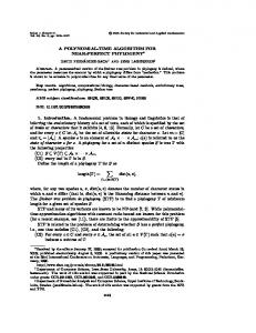
Figure 1: The context-free process X ! aY , Y ! aY Z , Y ! b, Z ! b

 P  V  (V [ T ) is a nite set of production rules, written X !  for (X; ) 2 P . We shall assume that some rule X !  exists in P for each variable X 2 V ; and  S 2 V is the start symbol. The norm of a variable X 2 V , written norm(X ), is the length of the shortest string of terminals which can be generated from X . A CFG is weakly normed i its start symbol has a nite norm, and it is normed i all of its variables have nite norm. A grammar is in Greibach normal form (GNF) i each of its production rules is of the form X ! a where a 2 T and  2 V . If each such  is of length at most k, then it is in k-GNF.

The class of CFGs in GNF corresponds to the class of processes de ned by guarded systems of recursive equations over the basic process algebra (BPA) of [1]. Every CFG in GNF in this sense de nes a (context-free) process as follows.

De nition 2.3 With the CFG (V; T; P; S ) in GNF we associate the process (V ; T; ?!; S ) a where there are no transitions leading from ", and X ?!  i X ! a is a production in P . The class of context-free processes is exactly that class of processes generated by CFGs in GNF.

As an example, consider the CFG given by the GNF rules X ! aY , Y ! aY Z , Y ! b and Z ! b. This grammar de nes the process depicted in Figure 1. This process (as well as its de ning grammar) is normed, with norm(X ) = 2 and norm(Y ) = norm(Z ) = 1. Clearly every normed CFG in GNF gives rise to a normed process. We can also see immediately the following basic fact regarding processes.

Lemma 2.4 norm( ) = norm() + norm( ). The notion of process equivalence in which we are interested is bisimulation equivalence [20] as de ned as follows. 4

De nition 2.5 Let (S; A; ?!; s0) be a process. A relation R  S  S is a bisimulation i whenever (; ) 2 R we have that a 0 a 0  if  ?!  then ?! for some 0 with (0; 0) 2 R; and a 0 a 0  if ?! then  ?!  for some 0 with (0; 0) 2 R.

 and are bisimilar, written   , i (; ) 2 R for some bisimulation R.

Lemma 2.6  is an equivalence relation. Proof Re exivity is established by demonstrating f(; ) :  2 S g to be a bisimulation; ? 1 symmetry is established by demonstrating R to be a bisimulation whenever R is; transitivity is established by demonstrating RS to be a bisimulation whenever R and S are.

These are all straightforward. 2 The main result on which we shall build regarding this process class, originally proved in [1], is given by the following.

Theorem 2.7 Bisimilarity is decidable for normed context-free processes. What we provide in this paper is a procedure of relatively low complexity for deciding bisimilarity of normed context-free processes. Speci cally, we x a CFG G = (V; T; P; S ) in GNF, and decide whether two given states  and of the process (V ; T; ?!; S ) given by De nition 2.3 are bisimilar. We shall rely on the following established results concerning bisimilar processes. s 0 s Lemma 2.8 If   and  ?!  for s 2 A then ?! 0 such that 0  0.

Proof Suppose that R is a bisimulation relating  and , and that a a1 a2  p = 0 .  = 0 ?! 1 ?!


?! p

Then we must have that a a1 a2 p = 0 = 0 ?! 1 ?!


?! p

with (i; i) 2 R for 0  i  p. Hence (0; 0) 2 R so 0  0.

Lemma 2.9   implies norm() = norm( ). 5

2

s Proof Suppose that norm() >s norm( ) and that ?! " with length(s) = norm( ). Clearly we cannot have that  ?! " so we cannot have that   . 2

The technique underlying our algorithm exploits properties of the sequential composition and decomposition of processes, as outlined in the following few facts. Firstly, we have a basic congruence result.

Lemma 2.10 If   and 0  0 then 0  0. o

n

Proof It is straightforward to show that (0 ; 0) :   ; 0  0 is a bisimulation. 2

More importantly, motivated by [19] we have a unique prime decomposition result for weakly normed (and hence normed) processes. To demonstrate this we rst prove a cancellation lemma.

Lemma 2.11 If   and is weakly normed, then   . n

o

Proof It is straightforward to show that (; ) :   ; norm( ) < 1 is a bisimu-

lation. 2 Notice that this fact fails to hold when is not weakly normed. For example, given X ! a and Y ! aY we have that XY  XXY but X 6 XX .

De nition 2.12  is prime (wrt ) i  6= " and   implies = " or = ". Theorem 2.13 Weakly normed processes have unique (up to ) prime decompositions. Proof Existence is established by induction on the norm. To establish uniqueness, suppose that 1


p  1


q are prime decompositions and that we have established the uniqueness of prime decompositions for all processes  with norm() < norm(1


p).

If p = 1 or q = 1 then we immediately have our result. a 0 Otherwise suppose that 12


p ?! 12


p is a norm-reducing transition, that is norm(012


p) < norm(12


p). a 0 1 2


q with 012


p  10 2


q, so by induction we must Then 1 2


q ?! have that p  q , Hence by Lemma 2.11 we have that 1


p?1  1


q?1 from which our result then follows by Lemma 2.10. 2 One further result concerning bisimilarity which we rely on pertains to Caucal bases, otherwise known as self-bisimulations [2]. 6

De nition 2.14 For any binary relation B over processes, let B be the congruence closure of B wrt sequential composition. B is a Caucal base i whenever (; ) 2 B we have that a 0 a 0  if  ?!  then ?! for some 0 with 0 B 0; and a 0 a 0  if ?! then  ?!  for some 0 with 0 B 0.

Lemma 2.15 If B is a Caucal base, then B is a bisimulation so B  . Proof We demonstrate that if  B then the two clauses given by De nition 2.5 hold true. The proof of this we carry out by induction on the depth of inference of  B . If  B follows from (; ) 2 B, then the result follows from B being a Caucal base. If  B follows by one of the congruence closure conditions, then the result easily follows

2

by induction.

3 Basic De nitions and Results In this section we provide the results which de ne and underlie the correctness of a deterministic algorithm for our decision problem. We start by assuming that we have a normed CFG (V; T; P; S ) in GNF, where the variables V = f X1; X2; : : :; Xn g are ordered by nondecreasing norm. The basic idea is to exploit the unique prime decomposition theorem by decomposing process terms suciently far to be able to establish or refute the equivalence which we are considering. Further, we try to construct these decompositions by a re nement process which starts with an overly generous collection of candidate decompositions. This is the motivation behind the following de nitions.

De nition 3.1 1. A base is a collection of pairs (Xj ; Xi ) where Xi ; Xj 2 V ,  2 V  , i  j , and satisfying norm(Xj ) = norm(Xi ) and = 0 whenever both (Xj ; Xi ) and (Xj ; Xi 0 ) are contained in B.

2. A base B is full i whenever Xj  Xi with j  i then (Xj ; Xi ) 2 B for some

 . In particular, (X; X ) 2 B for all X 2 V . 3. Let B  B be some relation satisfying   B whenever B is full. (We leave the actual de nition of B until later, at which time we shall con rm that these inclusions hold.)

7

Hence we are proposing that a base B consist of pairs (X; ) representing candidate decompositions, that is, such that X  . Our task then is to discover a full base which contains only semantically sound decomposition pairs. To do this, we start with a full but nite (and indeed small) base which we re ne iteratively whilst maintaining fullness. This re nement is as follows.

De nition 3.2 Given a base B, de ne the subbase Bb  B by: (X; ) 2 Bb i (X; ) 2 B and a a  if X ?! then  ?!

with B ; a a  if  ?!

then X ?! with B .

and

Lemma 3.3 If B is full then Bb is full. Proof If Xj  Xi with j  i, then by fullness of B we have (Xj ; Xi ) 2 B for some

 . a a If Xj ?!  then Xi ?!  with    and thus again by fullness of B we have  B . a a Similarly if Xi ?!  then Xj ?!  with    and thus  B . Hence (Xj ; Xi ) 2 Bb . 2 So we can iteratively apply this re nement to our nite full base, and be guaranteed that the process will stabilize at some full base B for which we can demonstrate that B = . This last result will follow from De nition 3.1(3) as well as the following.

Proposition 3.4 If Bb = B then B  . Proof B is contained in B , the congruence generated by B, so B must be a Caucal

base. Hence our result follows from Lemma 2.15. 2 We are thus simply left now with the task of constructing our initial base B0. This is achieved as follows.

De nitions 3.5 For each i and j in the range 1  i  j  n x some [Xj ]norm(X ) such that Xj ?! [Xj ]norm(X ) in length(s) = norm(Xi) norm-reducing steps. Let B0 be the collection of all such (Xj ; Xi [Xj ]norm(X )) pairs. i

i

i

Lemma 3.6 B0 is full. Proof If sXj  Xi with i  j , then (Xj ; Xi [Xj ]norm(X )) 2 B0 for some [Xj ]norm(X ) such that Xj ?! [Xj ]norm(X ) in length(s) = norm(Xi ) norm-reducing steps. But this norms reducing transition sequence can only be matched by Xi ?! . Hence we must have that [Xj ]norm(X )  , so B0 must be full. 2 i

i

i

8

i

De nition 3.7 Let Bi+1 = Bci, and let B be the the rst Bi+1 = Bi. We thus nally have our desired base B, and we are left to state our promised characterisation theorem.

Theorem 3.8 B = . Proof Immediate from De nition 3.1(3) and Proposition 3.4.

2

We have now accomplished our goal of de ning a deterministic procedure for deciding bisimilarity between normed processes: we simply iterate our re nement procedure on our nite initial base B0 until it stabilizes at our desired base B, and then test for B . However, we have not given an explicit algorithm for performing this procedure | indeed we have not even de ned our relation B , so we cannot even deduce that it is computable let alone decidable | so we cannot as yet remark on its complexity. This task is left for the next section.

4 A Polynomial Solution In this section we accomplish our goal by describing a deterministic implementation of our basic algorithm which runs in polynomial time. To start with, we x the problem domain: let (V; T; P; X1) be a CFG in k-GNF, with

V = fnX1; X2; : : :; Xn g o P = Xi ! aij ij : 1  i  n; 1  j  mi and such that the indices on the variables and productions are ordered by increasing norm so that norm(Xi )  norm(Xi+1 ) for each 1  i < n. Let m be the maximum value of mi, that is, the maximumnumber of rules associated with a single variable, and hence the maximum number of transitions evolving from any given state. Finally assume that the rst rule for each variable generates a norm-reducing transition, so that norm(Xi ) < norm(i1). (We can compute the norms of the variables by solving simple linear equations and thus transform our grammar into this form in polynomial time.) We want to decide, given ; 2 V , whether or not   . To do so, we start by computing B as in the previous section, and then determine if  B . The algorithm thus has three phases: the rst phase computes the initial base B0; the second phase computes the nal base B by iterating the re nement operation until it stabilizes; and the third phase decides if the two processes in question are related by B . We rst consider the complexity of computing a particular B0. In order to compute B0 we must compute [Xi]p, a term derived from Xi through p  norm(Xi) norm-reducing steps. In particular, these steps will be xed as those given by the rst rule for each Xi. A function for de ning []p for p  norm() is thus given as follows. 9

De nition 4.1 []0 def = 8 ;

[Xi]p def =

< :

[]p?norm(X ) if p  norm(Xi); [i1]p?1 if p < norm(Xi ): i

Some fundamental properties of this de nition are summarized as follows.

Lemma 4.2 a2


a []p in p norm-reducing steps. 1. For p  norm(),  a1?! p

2. []norm() = ".

3. For p  norm() and p + q  norm( ), [[]p ]q = [ ]p+q .

4. length([]p)  (j ? 1)(k ? 1) + length(), where j is the maximum index of a variable appearing in  (or 1, if  = "). In particular, length([Xi ]p )  (i ? 1)(k ? 1) + 1

5. Computing []p takes at most (j ? 1)k + length() steps, where j is the maximum index of a variable appearing in  (or 1, if  = "). In particular, [Xi ]p takes at most (i ? 1)k + 1 steps to compute.

Proof 1. By induction on p. Firstly, if p = 0 then the result is immediate. Otherwise let  = Xi . If p  q = norm(Xi) then +1


a 1


a a ?!  a?! [ ]p?q = []p. If p < norm(Xi) then q

q

p

a1 2


a [i1 ]p?1 = []p.  ?! i1 a?! 2. By induction on norm(). If  = " then the result is immediate. Otherwise let  = Xi . Then []norm() = [ ]norm( ) = ". p

10

3. By induction on norm( ). Firstly, if p = 0 then the result is immediate. Otherwise let  = Xi . If p  norm(Xi) then [[]p ]q = [[ ]p?norm(X ) ]q = [ ]p+q?norm(X ) = [ ]p+q. If p + q < norm(Xi ) then [[]p ]q = [[i1]p?1 ]q = [i1 ]p+q?1 = [ ]p+q. If p < norm(Xi)  p + q then [[]p ]q = [[i1]p?1 ]q = [i1 ]p+q?1 = [[i1]norm(X )?1 ]p+q?norm(X ) = [ ]p+q?norm(X ) = [ ]p+q. 4. By induction on p. Firstly, if p = 0 then the result is immediate. Otherwise let  = Xi . If p  norm(Xi) then length([]p) = length([ ]p?norm(X ))  (j ? 1)(k ? 1) + length() ? 1 (by induction.) If p < norm(Xi) then length([]p) = length([i1]p?1 )  (i ? 2)(k ? 1) + k + length() ? 1 (by induction)  (j ? 1)(k ? 1) + length(). 5. By induction on p. Firstly, if p = 0 then the result is immediate. Otherwise let  = Xi . If p  norm(Xi ), then the computation of []p takes one more step than the computation of [ ]p?norm(X ), which, by induction, takes at most (j ? 1)k + (length() ? 1) steps, giving the result. If p < norm(Xi), then []p takes one more step to compute than [i1]p?1, which, since i1 is a sequence of at most k variables with smaller norm | and hence indices | than Xi, by induction takes at most (i ? 2)k + k steps to compute, which gives us our result. i

i

i

i

i

i

i

Our basic algorithm for computing   then takes the following form. 11

2

1. Computenthe initial base B = B0: o B = (Xj ; Xi[Xj ]norm(X )) : 1  i  j  n i

2. Iterate the re nement procedure B = Bb until it stabilizes: Unmatched = ;;

repeat B = B n Unmatched; Unmatched = ;; for each (Xj ; Xi[Xj ]norm(X )) 2 B do if 9 1  q  mj such that 8 1  p  mi ajq =6 aip or jq 6B ip[Xj ]norm(X ) or 9 1  p  mi such that 8 1  q  mj ajq =6 aip or jq 6B ip[Xj ]norm(X ) n o then Unmatched = Unmatched [ (Xj ; Xi[Xj ]norm(X )) ; until Unmatched = ;; 3. Return  B . i

i

i

i

Using Lemma 4.2(5), we see that the cost of the rst phase is O(n3 k). For the second step, the outer loop may execute O(n2 ) times, as can the inner loop, and the body of this looping construct consists of O(m2) calculations of relations of the form B , where length( )  k (since the grammar is in k-GNF), and length()  nk (by Lemma 4.2(4) and since the grammar is in k-GNF). The cost of the algorithm is thus O(n4m2f (n; nk; (n + 1)k)), where f (n; q; l) is the cost of computing B  given that there are n variables, each (X; ) 2 B satis es length( )  q, and length( )  l. We are now ready to reveal the key to our polynomial algorithm, an appropriate de nition of B which has a polynomial complexity.

De nition 4.3 Let V = f X1; X2; : : :; Xn g. A function g : V ! V  is a decomposing function of order q if either g (Xi ) = Xi or g(Xi ) = Xj1 Xj2


Xj with 1  p  q and i > jr for each 1  r  p. p

Such a g can be extended to the domain V  in the obvious fashion by g (") = " and g(X) = g(X )g(). We can then de ne g () for  2 V  to be the limit of g t () as t ! 1; due to the restricted form of g we know that it must be eventually idempotent, that is, that this limit must exist. The notation g[X 7! ] denotes the function that agrees with g at all points in V except X , where its value is .

De nition 4.4 For base B and decomposing function g, de ne  gB by 12

 if g() = g( ) then the result is true.  Otherwise let Xi and Xj (with i < j ) be the leftmost mismatching pair. { If (Xj ; Xi ) 2 B then the result is given by  gB[X 7!X ] . { Otherwise the result is false. j

i

Finally, let B = Id B where Id is the identity function.

Lemma 4.5 B  B , and   B whenever B is full. Proof The rst part is easily con rmed, since for any g constructed by the algorithm computing B , X B g(X ) for each X 2 V . For the second part, suppose that   and at some point in our procedure for deciding  B we have that g() = 6 g( ), and that we have only ever updated g with mappings X 7! satisfying X  . Let Xi and Xj (with i < j ) be the leftmost mismatching pair. Then we must have Xj  Xi for some , so by fullness, we must have that (Xj ; Xi ) 2 B for some with Xj  Xi . So we cannot terminate our procedure for deciding  B with a false result, as the procedure will update g with this new semantically sound mapping and continue. 2

Lemma 4.6 Given a decomposing function g of order q, there is an algorithm which  decides if g () = g ( ) which runs in time O (nq)4 + (nq)2( length( )) for arbitrary ; 2 V . If g() 6= g( ) then the algorithm reports the leftmost mismatching pair (as required by De nition 4.4). Proof See Appendix A. 2 Computing  B requires at most n calculations of g() = g( ) for decomposing functions over n variables of order nk, where length( ) = (n + 1)k. Adding this all up gives us a complexity of O(n9 k4) for computing  B . Hence our algorithm for deciding bisimilarity of normed context-free processes runs in time O(n13m2k4), or in terms of the size jGj of the grammar (noting that jGj  nkm), O(jGj13).

5 Simple Context-Free Grammars It is a corollary of our main result that language equivalence of simple context-free grammars can be decided in polynomial time. A simple grammar is a context free grammar in Greibach normal form such that for any pair (X; a) consisting of a variable X and terminal a, there is at most one production of 13

the form X ! a. The equivalence problem for simple grammars was rst considered by Korenjak and Hopcroft [17], who presented a decision procedure with time complexity O(nv ), where n is the size of the grammar (i.e., the total length in symbols of all the productions) and v is the shortest word generated by the grammar. The time complexity was improved to O(n3 v) by Caucal [3]. Since v is in general exponential in n, the above decision procedures have, respectively, doubly exponential and singly exponential time complexities. To obtain a polynomial-time decision procedure we merely note that, in the case of simple grammars, language equivalence and bisimulation equivalence coincide. All that needs to be checked is that the relation of language equivalence on processes is a bisimulation. (The reverse inclusion is automatic, since bisimulation equivalence is always a re nement of language equivalence.) The key observation is that when a process de ned by a simple grammar undergoes a transition, the resulting process is uniquely determined by the action that has been performed. Thus language equivalence of simple grammars may be checked in polynomial time by the procedure presented in the previous section.

6 Conclusions We have demonstrated a polynomial-time algorithm for deciding bisimilarity between normed context-free processes. Previously, the best complexity bound, due to Huynh and Tian [15], put the problem in P2 = NPNP. Our approach is initially similar to their proof of membership in P2. Our contribution is to show that the NP-oracle calls used in their proof for comparing unique decompositions (ie, deciding g() = g( )) can in fact be replaced by calls to a polynomial-time subroutine. This enhancement allows us to dispense with the inner (universal) quanti cation implicit in the P2 algorithm. The outer (existential) quanti cation is dismissed by employing a deterministic procedure for constructing the decomposition function g. The original motivation for the work presented here was to nd an ecient deterministic implementation of the problem. This aspect is explored in [11], where we explore an optimised version of the algorithm underlying the co-NP algorithm. The algorithm runs in time which is linearly bounded by the norm of the processes being compared, and although this is potentially exponential in the size of the problem, it is still worth considering to be ecient. Indeed, with the optimisations described in [11], it is reasonable to expect that our polynomial-time algorithm may well be less ecient in practice than this exponential algorithm. Very recently the authors have also developed a polynomial-time algorithm to decide bisimulation equivalence of an analogue of BPA (called BPP) in which commutative (parallel) composition replaces noncommutative (sequential) composition [10]. This result improves considerably on the time complexity of decision procedures that can be extracted from from the tableau systems of Christensen, Hirshfeld and Moller [4, 5].

14

References [1] J.C.M. Baeten, J.A. Bergstra and J.W. Klop. Decidability of bisimulation equivalence for processes generating context-free languages. In Proceedings of PARLE 87, J.W. de Bakker, A.J. Nijman, P.C. Treleaven (eds), Lecture Notes in Computer Science 259, pp93{114, Springer-Verlag, 1987. [2] D. Caucal. Graphes canoniques des graphes algebriques. Informatique Theorique et Applications (RAIRO) 24(4), pp339{352, 1990. [3] D. Caucal. A fast algorithm to decide on the equivalence of stateless DPDA. Informatique Theorique et Applications (RAIRO) 27(1), pp23{48, 1993. [4] S. Christensen, Y. Hirshfeld and F. Moller. Decomposability, decidability and axiomatisability for bisimulation equivalence on basic parallel processes. In Proceedings of LICS93. IEEE Computer Society Press, 1993. [5] S. Christensen, Y. Hirshfeld and F. Moller. Bisimulation equivalence is decidable for basic parallel processes. In Proceedings of CONCUR93, E. Best (ed), Lecture Notes in Computer Science 715, pp143{157, Springer-Verlag, 1993. [6] S. Christensen, H. Huttel and C. Stirling. Bisimulation equivalence is decidable for all context-free processes. In Proceedings of CONCUR 92, W.R. Cleaveland (ed), Lecture Notes in Computer Science 630, pp138{147. Springer-Verlag, 1992. [7] R.J. van Glabbeek. The linear time-branching time spectrum. In Proceedings of CONCUR 90, J. Baeten, J.W. Klop (eds), Lecture Notes in Computer Science 458, pp278{297. Springer-Verlag, 1990. [8] J.F. Groote. A short proof of the decidability of bisimulation for normed BPA processes. Information Processing Letters 42, pp167{171, 1991. [9] J.F. Groote and H. Huttel. Undecidable equivalences for basic process algebra. Information and Computation, 1994. [10] Y. Hirshfeld, M. Jerrum and F. Moller, A polynomial algorithm for deciding bisimulation equivalence of normed Basic Parallel Processes, Department of Computer Science Research Report, University of Edinburgh. (In preparation.) [11] Y. Hirshfeld and F. Moller. A fast deterministic algorithm for deciding bisimilarity of normed context-free processes. Department of Computer Science Research Report. University of Edinburgh, 1994. [12] Y. Hirshfeld and F. Moller. Algorithms for Normed Processes. In Proceedings of the VIII Ban Higher-Order Workshop, August, 1994. [13] J.E. Hopcroft and J.D. Ullman. Introduction to Automata Theory, Languages, and Computation. Addison Wesley, 1979. 15

[14] H. Huttel and C. Stirling. Actions speak louder than words: proving bisimilarity for context-free processes. In Proceedings of LICS'91, IEEE Computer Society Press, pp376{386, 1991. [15] D.T. Huynh and L. Tian. Deciding bisimilarity of normed context-free processes is in P2. Journal of Theoretical Computer Science 123, pp183{197, 1994. [16] D.E. Knuth, J.H. Morris, and V.R. Pratt, Fast pattern matching in strings, SIAM Journal on Computing 6 (1977), pp323{350. [17] A. Korenjak and J. Hopcroft. Simple deterministic languages. In Proceedings of 7th IEEE Switching and Automata Theory conference. pp36{46, 1966. [18] R. Milner. Communication and Concurrency. Prentice Hall, 1989. [19] R. Milner and F. Moller. Unique decomposition of processes. Journal of Theoretical Computer Science 107, pp357{363, 1993. [20] D.M.R. Park. Concurrency and Automata on In nite Sequences. Lecture Notes in Computer Science 104, pp168{183, Springer Verlag, 1981. [21] L.J. Stockmeyer. The polynomial time hierarchy. Journal of Theoretical Computer Science 3, pp1{22, 1977.

A Proof of Lemma 4.6 We start by reminding ourselves of the conditions of the lemma. Let V = f X1 ; X2; : : :; Xn g, and g : V !V satisfy either g(Xi) = Xi or g(Xi ) = Xj1 Xj2


Xj with 1  p  q and i > jr for each r in the range 1  r  p. Extend the de nition of g to the domain V  in the obvious fashion by g(") = " and g(X) = g(X )g(). Finally de ne g() for  2 V  to be the limit of gt() as t ! 1. We shall begin by assuming that this function g maps a single variable to at most two variables. This is justi ed, as given g(X ) = Y1Y2


Yp with 2 < p  q, we can introduce p ? 2 < q new variables W1; : : :; Wp?2 and rede ne g by g(X ) = Y1W1, g(Wp?2) = Yp?1Yp, and g(Wi?1) = YiWi for 2  i < p ? 2. Thus we need only introduce O(nq) auxiliary variables, and this transformation does not change the value of g() for any  2 V . In the sequel, let n denote the total number of variables after this reduction to what is essentially Chomsky normal form, and let V refer to this extended set of variables. It thus remains for us to demonstrate if g() = g( ) for arbitrary  an algorithm for deciding  ; 2 V  which runs in time O n4 + n2( length( )) . Furthermore, in the case that g() 6= g( ), the algorithm must return the leftmost pair (Xi; Xj ) with i > j at which there is a mismatch. p

16

 = g(X ) = g(Y )

= g(Z ) First symbol of , and ith of  Figure 2: A alignment of  that spans and

6

We say that the positive integer r is a period of the word  2 V  if 1  r  length(), and the symbol at position p in  is equal to the symbol at position p + r in , for all p in the range 1  p  length() ? r. Our argument will be easier to follow if the following lemma is borne in mind; we state it in the form given by Knuth, Morris and Pratt [16, Lemma 1].

Lemma A.1 If r and s are periods of  2 V , and r + s  length() + gcd(r; s), then

gcd(r; s) is a period of .

Proof See [16, Lemma 1]; alternatively the lemma is easily proved from rst principles. 2

For ; 2 V , we shall use the phrase alignment of  against to refer to a particular occurrence of  as a subword of . Note that if two alignments of  against overlap, and one alignment is obtained from the other by translating  through r positions, then r is a period of . Suppose X; Y; Z 2 V , and let  = g(X ), = g(Y ), and = g(Z ). Our strategy is to determine, for all triples X , Y , and Z , the set of alignments of  against that include the rst symbol of (see Figure 2). Such alignments, which we call spanning, may be speci ed by giving the index i of the symbol in  that is matched against the rst symbol in . It happens that the sequence of all indices i that correspond to valid alignments forms an arithmetic progression. This fact opens the way to computing all alignments by dynamic programming: rst with X = X1 and Y; Z ranging over V , then with X = X2 and Y; Z ranging over V , and so on.

Lemma A.2 Let ;  2 V  be words, and A be the set of all indices i such that there exists

an alignment of  against  in which the ith symbol in  is matched to a distinguished symbol in . Then the elements of A form an arithmetic progression.

Proof Assume that there are at least three alignments, otherwise there is nothing to

prove. Consider the leftmost, next-to-leftmost, and rightmost possible alignments of  against . Suppose the next-to-leftmost alignment is obtained from the leftmost by translating  though r positions, and the rightmost from the next-to-leftmost by translating  through s positions. Since r and s satisfy the condition of Lemma A.1, we know that gcd(r; s) is a period of ; indeed, since there are by de nition no alignments between the leftmost and next-to-leftmost, it must be the case that r = gcd(r; s), i.e., that s is a multiple of r. Again by Lemma A.1, any alignment other than the three so far considered must also have the property that its oset from the next-to-leftmost is a multiple of r. 17

 g(Yj(i))



6 g(Yj(+1i) )

p Figure 3: Trapping an alignment

Thus the set of all alignments of  against  can be obtained by stepping from the leftmost to the rightmost in steps of r. This completes the proof, but it is worth observing for future reference, that in the case that there are at least three alignments of  against  containing the distinguished symbol, then  must be periodic, i.e., expressible in the form  = %k , where k  2 and  is a (possibly empty) strict initial segment of %. 2 In the course of applying the dynamic programming technique to the problem at hand, it is necessary to consider not only spanning alignments of the form illustrated in Figure 2, but also inclusive alignments: those in which  = g(X ) appears as a subword of a single word = g(Y ). Fortunately, alignments of this kind are easy to deduce, once we have computed the spanning alignments.

Lemma A.3 Suppose spanning alignments of  = g(X ) against = g(Z ) and 0 = g(Z 0) have been pre-computed for a particular X and all Z; Z 0 2 V . Then it is possible,

in polynomial time, to compute, for any Y and any distinguished position p in = g (Y ), all alignments of  against that include p.

Proof Consider the sequence n

o

g(Y1(0)) ;

n

o

g(Y1(1)); g(Y2(1)) ;

n

o

g(Y1(2)); g(Y2(2)); g(Y3(2)) ; : : :

of partitions of = g(Y ), obtained by the following procedure. Initially, set Y1(0) = Y . Then, for i  1, suppose that g(Yj(i?1)) is the block of the (i ? 1)th partition that contains the distinguished position p, and let Z = Yj(i?1) be the symbol generating that block. Let the ith partition be obtained from the (i ? 1)th by splitting that block into two | g(Z 0) and g(Z 00) | where g(Z ) = Z 0Z 00. The procedure terminates when g(Z ) = Z , a condition which is bound to hold within at most n steps. Observe that, aside from in the trivial case when length() = 1, any alignment of  containing position p will be at some stage(i\trapped," so that the particular occurrence of the subword  in is contained in )  (i) (i) (i)    g (Yj ) g (Yj+1), but not in g (Yj ) or g (Yj+1 ) separately (see Figure 3). For each such situation, we may compute the alignments that contain position p. (By Lemma A.2, these form an arithmetic progression.) Each alignment of  that includes p is trapped at least once by the partition re nement procedure. The required result is the union of at most n arithmetic progressions, one for each step of the re nement procedure. Lemma A.2 guarantees that the union of these arithmetic progressions will itself be an 18

 = g(Y )

6

 = g(X )

6

6

= g(Z )

.

0 = g(X 0) p 00 = g(X 00) Figure 4: Dynamic programming: inductive step 0

00

6

6

p0 p Figure 5: Dynamic programming: the leftmost alignment arithmetic progression. Thus the result may easily be computed in time O(n) by keeping track of the leftmost, next-to-leftmost, and rightmost points. 2 The necessary machinery is now in place, and it only remains to show how spanning alignments of the form depicted in Figure 2 may be computed by dynamic programming, rst for X = X1, then X = X2, and so on, up to X = Xn . If g(X ) = X , the task is trivial, so suppose g(X ) = X 0X 00. The function g induces a natural partition of  = g(X ) into 0 = g(X 0) and 00 = g(X 00); suppose it is 00 that includes p, the rst symbol in (see Figure 4.) We need to discover the valid alignments of 0 against , and conjoin these with the spanning alignments | that we assume have already been computed | of 00 against and . Consider the leftmost valid alignment of 00 and let p0 be the position immediately to the left of 00 (see Figure 5). We distinguish two kinds of alignments for  = 000. The alignment of 0 against includes position p0. These alignments can be viewed as conjunctions of spanning alignments of 00 (which are precomputed) with inclusive alignments of 0 (which can be computed on demand using Lemma A.3). The valid alignments in this case are thus an intersection of two arithmetic progressions, which is again an arithmetic progression. Case I.

The alignment of 0 against does not includes position p0, i.e., lies entirely to the right of p0. If there are just one or two spanning alignments of 00 against and , then we simply check exhaustively, using Lemma A.3, which, if any, extend to alignments of  against . Otherwise, we know that 00 has the form %k  with k  2, and  a strict initial segment of %; choose % to minimise length(%). A match of 00 will extend to a match of  only if 0 = 0%m, where 0 is a strict nal segment of %. (Informally, 0 is a smooth continuation of the periodic word 00 to the left. Thus either every alignment of 00 extends to one of  = 000, or none does, and it is easy to determine which is the case. As in Case I, the result is an arithmetic progression. Case II.

The above arguments were all for the situation in which it is the word 00 that contains p; the other situation is covered by two symmetric cases | Case I0 and Case II0 | which are 19

as above, but with the roles of 0 and 00 reversed. To complete the inductive step of the dynamic programming algorithm, it is only necessary to take the union of the arithmetic progressions furnished by Cases I, II, I0, and II0: this is straightforward, as the result is known to be an arithmetic progression by Lemma A.2. At the completion of the dynamic programming procedure, we have gained enough information to check arbitrary alignments, both spanning and inclusive, in polynomial time. From there it is a short step to the promised result.

Proposition A.4 There is a polynomial-time algorithm for deciding g() = g( ) for arbitrary ; 2 V . In the case that g  () = 6 g( ), the algorithm returns the leftmost

position at which there is a mismatch.

Proof Let = Y1Y2 : : :Ys . Apply the partition re nement procedure used in the proof

of Lemma A.3 to the word  to obtain a word 0 = X1X2 : : :Xr with the property that each putative alignment of g(Xi ) against the corresponding g(Yj ) or g(Yj ) g(Yj+1 ) is either inclusive or spanning. This step extends the length of  by at most an additive term length( ) n. Now test each Xi either directly, using the precomputed spanning alignments, or indirectly, using Lemma A.3. In the case that g() 6= g( ), determine the leftmost symbol Xi such that g(Xi ) contains a mismatch. If g(Xi) = Xi we are done. Otherwise, let g(Xi) = ZZ 0, and test whether g(Z ) contains a mismatch: if it does, recursively determine the leftmost mismatch in g(Z ); otherwise determine the leftmost mismatch in g(Z 0). During the dynamic programming phase, there are O(n3) subresults to be computed (one for each triple X; Y; Z 2 V ), each requiring time O(n); thus the time-complexity of this phase is O(n4). Re ning the input  to obtain 0, and  checking alignments of individual 0 2 symbols of  takes further time O n ( length( )) . The overall time complexity of a  4 2 nave implementation is therefore O n + n (length( )) . 2

20