alence of normed context-free processes worked in O(n13) time. We give ... algorithm for bisimilarity on normed context-free processes, thus improving pre-.
Faster Algorithm for Bisimulation Equivalence of Normed Context-Free Processes S�lawomir Lasota� and Wojciech Rytter�� Institute of Informatics, Warsaw University, Warsaw, Poland
Abstract. The fastest known algorithm for checking bisimulation equivalence of normed context-free processes worked in O(n13 ) time. We give an alternative algorithm working in O(n8 polylog n) time, As a side effect we improve the best known upper bound for testing equivalence of simple context-free grammars from O(n7 polylog n) to O(n6 polylog n).
1
Introduction
Equivalence checking, that is determining whether two systems are equal under a given notion of equivalence, is an important verification problem with a long history. In this paper we consider systems described by context-free grammars. It is well known that language equivalence is undecidable in this class [1]. A decidability result was obtained by Korenjak and Hopcroft [12] for a restricted class of deterministic context-free grammars (simple grammars). Remarkably, the language containment is undecidable even for simple grammars [6]. In the context of process algebras, a grammar may be considered as a description of a transition graph rather than a language. The adequate concept of equivalence is then bisimilarity (bisimulation equivalence), a notion strictly finer than language equivalence. For graphs generated by context-free grammars, called context-free processes, bisimilarity is known to be decidable due to the result of [5]. It has also been demonstrated that bisimilarity is the only equivalence in van Glabbeek’s spectrum [7] which is decidable for context-free processes. This places bisimilarity in a very favourable position. Historically the first decision procedure for bisimilarity on infinite-state systems was given by [3] for a class of normed context-free processes, those defined by grammars in which, roughly, each nonterminal generates at least one word. Clearly, language equivalence is still undecidable in this class, as normedness assumption does not facilitate testing language equality. As language equivalence and bisimilarity coincide on deterministic graphs (in fact, the whole van Glabbeek’s spectrum collapses), the result of [3] was a strict extension of [12]. Later, decidability was extended to all context-free processes [5]. In the case of normed context-free processes, a number of simplifications of the proof of [3] appeared [4,10], relying on particular decomposition properties of �
��
Partially supported by the Polish Kbn grant No. 4 T11C 042 25 and by European Community Research Training Network Games. Supported by the Polish Kbn grant No. 4 T11C 044 25.
R. Kr´ aloviˇ c and P. Urzyczyn (Eds.): MFCS 2006, LNCS 4162, pp. 646–657, 2006. c Springer-Verlag Berlin Heidelberg 2006 �
Faster Algorithm for Bisimulation Equivalence
647
bisimilarity, and yielding an exponential upper bound for bisimilarity checking. A side effect was an improvement for the equivalence of simple grammars, compared to the complexity of the algorithm of [12] which was O(nv ), where n is the length of the grammar and v is the length of the shortest word generated, in general exponential in n. Independently, Caucal [4] proposed an algorithm for equivalence of simple grammars working in time O(n3 v). Huynh and Tian [11] did a next step and proved that complexity of bisimilarity is in NPNP , the second level of the polynomial hierarchy. A first polynomial-time procedure was finally presented by Hirshfeld, Jerrum and Moller [9]. The algorithm in [9] works in time O(n13 ) and is hence not satisfactory from the practical point of view. This motivated a further research: in [2] an O(n7 polylog n) time algorithm was proposed for the equivalence of simple grammars. In this paper we report a further progress: we give an O(n8 polylog n) time algorithm for bisimilarity on normed context-free processes, thus improving previous O(n13 ) time of [9]. We believe that our algorithm is conceptually simpler than that of [9]. It is based on the following two insights. First, we avoid an iterative computation of bisimilarity, by a chain of approximants of the greatest fixed point; instead, we are able to reduce the problem of computing the greatest bisimulation to the problem of finding the greatest solution of certain system of boolean equations, and use the linear-time procedure to find this solution. Secondly, we contribute to the algorithmic theory of compressed strings: we develop a fast algorithm for an auxiliary problem on strings called the First Mismatch Problem, working in O(n5 polylog n) time. As a direct corollary, the equivalence of simple grammars can be decided in O(n6 polylog n) time, which beats the complexity of the (fastest known) algorithm of [2]. Context-Free Processes and Bisimilarity. Let Σ be a finite alphabet and V = {X1 , . . . , Xm } a finite set of variables. By a process definition Δ we mean a a finite set of rules of the form: X −→ α, with a ∈ Σ and α ∈ V∗ . Such process definitions are usually called in the literature Basic Process Algebra, or Context-Free Processes. The explanation of the latter is that each rule can be seen as a production X −→ aα of a context-free grammar in Greibach normal form. Elements of V∗ are called here processes; a variable X can be seen as an elementary process. Δ defines a transition system: its states are processes α ∈ V∗ ; and for each a ∈ Σ, there is a transition relation containing triples (α, a, β), where a ∈ Σ a and α, β ∈ V∗ , written α −→ β. The transition relations are defined by a prefix a a rewriting: Xβ −→ αβ whenever Δ contains a rule X −→ α, and β ∈ V∗ . Definition 1. Given a binary relation R over V∗ , we say that a pair (α, β) of processes satisfies expansion in R if a
a
– whenever α −→ α� , there exists some β � with β −→ β � and (α� , β � ) ∈ R; and a a – whenever β −→ β � , there exists some α� with α −→ α� and (α� , β � ) ∈ R. A binary relation S satisfies expansion in R if each pair (α, β) ∈ S does. A relation R is a bisimulation if it satisfies expansion in itself. We say that α and β are bisimilar, denoted by α ∼ β, if (α, β) belongs to some bisimulation.
648
S. Lasota and W. Rytter
Assume that Δ is normed, i.e., for each variable X ∈ V∗ there is a finite sequence a1 ak X −→ α1 . . . −→ αk = ε leading from X to the empty process ε. By |X| denote the smallest length of such sequence and call it the norm of X (intuitively, |X| is the length of the shortest word generated from X). We consider the following Normed-BPA-Bisim Problem: Instance: A normed Δ and X, Y ∈ V with |X| = |Y |, X �= Y . Question: Is X ∼ Y ? A more general problem of checking whether α ∼ β, for any α, β ∈ V∗ , can be � (n)) for O(f (n) polylog n) easily reduced to the above one. We use notation O(f in the sequel. The size of Δ, denoted by n, is the sum of lengths of all the rules in Δ. Our main result is the following: � 8 ). Theorem 1. Normed-BPA-Bisim Problem can be solved in time O(n
2
Terminology and Tools Used in the Main Algorithm
The normedness assumption implies that each variable has at least one rule in Δ. We extend additively the norm to all processes: |ε| := 0, |Xα| := |X| + |α|. a1 ak . . . −→ ε leading Bisimilarity preserves norm, as a sequence of transitions X −→ to ε must be necessarily matched by a sequence leading to ε as well: Proposition 1. If α ∼ β then |α| = |β|. Let Σ, V and Δ be fixed from now on. We assume that the variables in V are ordered so that |Xi | ≤ |Xj | whenever i < j. It is easy to show the following: � Proposition 2. Norms of all variables can be computed in time O(n). The following fact is easily derived from the unique decomposition property [9]. Lemma 1. If αα� ∼ ββ � and |α| ≥ |β| then for some γ, α ∼ βγ and γα� ∼ β � . As s direct corollary we get a cancellation property: Lemma 2. If γα ∼ γβ then α ∼ β. We will need a notion of base, which is a slight adaptation of [9]. Intuitively, it describes ways of decomposing an elementary process into smaller ones: Definition 2. A base is a set B of pairs (Xj , Xi γ), at most one for each pair (Xj , Xi ), such that i < j, γ ∈ V∗ and |Xj | = |Xi γ|. A base is full iff whenever Xj ∼ Xi β, for j > i, then (Xj , Xi γ) ∈ B, for some γ ∼ β. Note that whenever (Xj , Xi γ) ∈ B then necessarily Xi γ ∈ {X1 , . . . , Xj−1 }+ . In the sequel we rely on the following lemma proved in [9]: Lemma 3. A full base B0 can be constructed, in time O(n3 ), such that the length of γ is O(n), for each (Xj , Xi γ) ∈ B0 . Furthermore, B0 contains a pair (Xj , Xi γ) for each i, j such that j > i.
Faster Algorithm for Bisimulation Equivalence
649
Remark 1. By cancellation, if Xj ∼ Xi γ, then γ is unique up to bisimilarity. Basing on this observation, the construction of B0 is by inspecting an arbitrarily chosen sequence of |Xi | norm-reducing moves from Xj . Any process obtained at the end of such a sequence is a good candidate for γ. Remark 2. Note that B0 , being full, contains all pairs (Xj , Xi ) with Xj ∼ Xi . Fix the full base B0 from now on. Pairs (Xj , Xi γ) ∈ B0 we call decomposition pairs, or d-pairs in short. A d-pair (Xj , Xi γ) will be denoted by zji . In the sequel we will treat the d-pairs as boolean variables. The basic intuition will be that zji = true just in case when Xj ∼ Xi γ holds. We will also build the positive boolean formulas on top of d-pairs, by boolean connectives ∧, ∨ and symbols true, false (no negation). The empty conjunction (disjunction) is allowed as a formula and understood as true (false, respectively). A valuation is a mapping v from B0 to {true, false}. We extend valuations to formulas in the obvious way. Definition 3. A boolean equation system is a set of equations of the form zji = ψji , one for each zji ∈ B0 , where ψji is a positive boolean formula with variables from B0 . A solution is any valuation v such that v(zji ) = v(ψji ) for each zji ∈ B0 . Valuations are in one-to-one correspondence with subsets of B0 : for B ⊆ B0 , a corresponding valuation vB assigns true to a variable zji if and only if zji ∈ B. ¯ start with B = B0 Each boolean equation system has the greatest solution B: and iteratively update B by removing zji from B if vB (ψji ) = false, until B ¯ A relevant observation is a folklore (see e.g. [8]): eventually stabilizes yielding B. Lemma 4. The greatest solution of a boolean equation system can be computed in time linear wrt. the size of the system. The overall idea underlying the algorithm is as follows. Bisimilarity is the greatest bisimulation, i.e., ∼ satisfies expansion in itself. Hence, by Knaster-Tarski fixpoint theorem, it is also the greatest fixed point: α ∼ β if and only if (α, β) satisfies expansion in ∼. One crucial insight is that computing this greatest fixed point can be reduced to finding the greatest solution of certain system of boolean equations. Another insight is that the system of equations can be constructed effectively (due to Lemma 5 below). These two insights allowed us � 8 ). to obtain an algorithm working in time O(n Consider any sub-base B ⊆ B0 and two processes α, β ∈ V∗ of equal norm. We write α =B β if α and β can be shown equal by applying any number of substitutions Xj �−→ Xi γ, where (Xj , Xi γ) ∈ B. Formally: Definition 4. For B ⊆ B0 , let =B be the smallest symmetric relation over processes containing all identical pairs α =B α and such that if (Xj , Xi γ) ∈ B and αXi γβ =B δ then αXj β =B δ.
650
S. Lasota and W. Rytter
Example 1. If |A| > |B| > |C| > |D| > |E| and B0 = {(A, BBD), (A, ECEB), (C, DE), (B, CD), (B, DED), . . .} then we have AEBBBD =B BBCCDA for B = {(A, BBD), (B, CD), (C, DE)}, due to the derivations of the same string: A=BBD
B=CD
AEBBBD −−−−→ BBDEBBBD −−−→ BBDECDBBD, C=DE
A=BBD
BBCCDA −−−→ BBDECDA −−−−→ BBDECDBBD. Note that B is inclusion-minimal, i.e., there is no B � � B with AEBBBD =B � BBCCDA. As B0 contains a pair (Xj , Xi γ) for each i and j with j > i, it follows that for α, β of equal norm some sub-base B with α =B β always exists; in particular α =B0 β. The relevant issue will be to find such B possibly small. For future reference, let B∼ ⊆ B0 be the set of all d-pairs (Xj , Xi γ) satisfying Xj ∼ Xi γ. Definition 5. We say that B is a matching sub-base for α, β iff it is an inclusion-minimal subset of B0 such that (i) α =B β and (ii) α ∼ β implies B ⊆ B∼ . In particular, by inclusion-minimality the matching sub-base for α, α is ∅. Condition (ii) says that a bisimilar pair can be shown equal by using only bisimilar substitutions. This property will follow by the unique decomposition (cf. Lemma 1) and by our intricate construction of the sub-base in the proof of Lemma 5. The proof of the lemma is postponed to Section 4. Lemma 5. For any processes α, β of length O(n) with |α| = |β|, we can compute � 6 ) time a matching sub-base Bα,β containing O(n) d-pairs. in O(n
3
The Main Algorithm
Basing on Bα,β , we define a matching formula for α, β, denoted by φα,β , as follows: if |α| = |β|, then φα,β is a conjunction of all d-pairs zji belonging to Bα,β , otherwise φα,β is false. In the algorithm we construct a boolean equation system containing an equation zji = ψji for each zji and then apply Lemma 4. The intuition is that formula ψji expresses the property that the d-pair zji satisfies expansion in ∼. However, instead of directly referring to α ∼ β in ψji , we will prefer to use formulas φα,β as subformulas in ψji , relying on condition (ii) in Definition 5. Let zji = (Xj , Xi γ). The formula ψji is defined as follows: ���� �� � (1) ψji = φβ,αγ ∧ φβ,αγ , a
β
α
α a
β
where a ranges over Σ, α ranges over {δ : Xi −→ δ ∈ Δ} and β ranges over a {δ : Xj −→ δ ∈ Δ}.
Faster Algorithm for Bisimulation Equivalence
651
Example 2. As an illustration, consider Δ containing variables X1 , . . . , X7 and c a the rules X5 −→ X1 , X7 −→ X5 , etc., as shown in the picture: a
{ & GFED @ABC X5 kf J
a
a
a
+ GFED x @ABC X4 f
c c a
c
@ABC GFED X1
b
GFED @ABC X7 a
c
a
� @ABC GFED X3
b
� @ABC GFED X6
a
@ABC GFED X2
a
a,c a,c
�� � + ε j
a
Δ is essentially finite-state. All variables have norm 1 except |X7 | = |X6 | = 2. Let B0 = {z76 = (X7 , X6 ), z72 = (X7 , X2 X5 ), z65 = (X6 , X5 X4 ), z64 = (X6 , X4 X4 ), z62 = (X6 , X2 X4 ), z54 = (X5 , X4 ), z32 = (X3 , X2 ), . . .}. B∼ = {(X3 , X1 ), (X5 , X4 ), (X7 , X6 ), (X6 , X2 X4 ), (X7 , X2 X5 )}. For instance, the equation for z76 is: � � � � � � � � z76 = φX5 ,X4 ∨φX5 ,X6 ∧ φX6 ,X4 ∨φX6 ,X6 ∧ φX6 ,X4 ∨φX5 ,X4 ∧ φX6 ,X6 ∨φX5 ,X6 . a
a
The first conjunct describes possible matchings for X7 −→ X5 , by X6 −→ X4 or a a X6 −→ X6 ; the second conjunct describes possible matchings for X7 −→ X6 , etc. Note for instance that φX5 ,X4 = z54 . Furthermore φX6 ,X6 = true as BX6 ,X6 = ∅; and φX5 ,X6 = false as |X5 | �= |X6 |. After simplification we derive: z76 = z54 . Similarly we derive: � � � � � � � � z54 = z54 ∧ z51 ∨ z31 ∧ z54 ∨ z43 ∧ z31 ∨ z43 ∧ z51 ∨ z54 . The greatest solution of the equation system is {z31 , z54 , z76 , z62 , z72 }. Algorithm Normed-BPA-Bisim(Δ, X, Y );
// |X| = |Y |
(1) compute a full base B0 ; // c.f. Lemma 3 (2) for each (Xj , Xi γ) ∈ B0 and a ∈ Σ do a a for each Xj −→ β and Xi −→ α in Δ do compute the formula φβ,αγ ; (3) for each zji = (Xj , Xi γ) ∈ B0 do construct the boolean expression (1); // this yields a boolean equation system S ¯ ⊆ B0 of S; (4) compute the greatest solution B ¯ (5) return [(X, Y ) ∈ B].
652
S. Lasota and W. Rytter
� 8 ). Lemma 6. The algorithm works in time O(n Proof. Step (1) requires time O(n3 ), by Lemma 3. The total number of invocations of the procedure computing φβ,αγ in step (2) is O(n2 ). Hence, step (2) � 8 ), by Lemma 5, and this is dominating the total can be completed in time O(n cost. The size of the boolean equation system built in step (3) is O(n3 ): indeed, the length of each subformula φβ,αγ is O(n), and there is a quadratic number of such formulas in the right-hand sides of equations. The equation system can be constructed in time O(n3 ) and its greatest solution can be computed in the same time, by Lemma 4. �
Lemma 7. The algorithm is correct. ¯ which is shown Proof. Correctness follows directly from the equality B∼ = B, below in two steps. ¯ first. Denote by ψji the right-hand side of equation (1) for We show B∼ ⊆ B ¯ zji = (Xj , Xi γ). B, as the greatest solution of the equation system, is the greatest subset B ⊆ B0 such that zji ∈ B (i.e., vB (zji ) = true) implies vB (ψji ) = true. Hence we will only show that zji ∈ B∼ (i.e, Xj ∼ Xi γ) implies vB∼ (ψji ) = true. Indeed. If Xj ∼ Xi γ then this pair satisfies expansion in ∼. Consider any pair a a β ∼ αγ relevant for the expansion, with Xj −→ β and Xi −→ α for some a. By point (ii) in Definition 5 we know that all d-pairs appearing in the matching formula φβ,αγ are bisimilar. As this applies to any pair β ∼ αγ, the right-hand side formula ψji is true under valuation vB∼ , as required. ¯ ⊆ B∼ . Consider any solution B of the equation system Now we will prove B and any d-pair zji = (Xj , Xi γ) ∈ B. Thus the right-hand side ψji evaluates to true under valuation vB . Consider any matching formula φβ,αγ appearing in ψji . If it is true under valuation vB then Bβ,αγ ⊆ B and hence β =B αγ, by point (i) in Definition 5. Hence, by the very construction of ψji on top of the matching formulas φβ,αγ it follows that (Xj , Xi γ) satisfies expansion in =B . B
But =B is clearly contained in ≡, the smallest congruence containing B. As the d-pair z was chosen arbitrarily, we have shown that B satisfies expansion B
in ≡, i.e., B is a so called Caucal base, or self-bisimulation [4]. By a standard B
argument ≡⊆∼, and hence B ⊆ B∼ . As all this was said for an arbitrary solution, ¯ ⊆ B∼ as required. in particular B �
4
Computing a Matching Sub-base
This section contains the construction of sub-bases Bα,β and the proof of Lemma 5. To this aim we need to refine the concept of base a little bit further. Definition 6. Aproduction isanypair(Xi , γ),written Xi → γ,suchthat |Xi | = |γ| A decomposition grammar and γ ∈ {X1 , . . . , Xi−1 }+ . (d-grammar) G is any set of productions Xi → γ, at most one for each variable Xi . Let V(G) denote the set of all Xi such that (Xi → γ) ∈ G for some γ. Variables in V(G) and V \ V(G) are called nonterminal and terminal symbols, respectively.
Faster Algorithm for Bisimulation Equivalence
653
Each nonterminal Xi has precisely one production, hence generates a single nonempty word G(Xi ) ∈ (V \ V(G))+ . We extend this to words α ∈ V∗ in the obvious way and write G(α) for the single word in (V \ V(G))∗ generated from α. A d-grammar G induces an equivalence =G over V∗ : α =G β iff α and β generate the same word, i.e., G(α) = G(β). Assume |α| = |β| hence |G(α)| = |G(β)|. One of G(α), G(β) can not be a proper prefix of the other. Hence, if α �=G β, the words G(α) and G(β) must have the left-most mismatching pair of variables. Formally: there is some i, j, γ such that i �= j, γXi is a prefix of G(α) and γXj is a prefix of G(β). W.l.o.g. assume i < j. The pair (Xj , Xi ) is called the first mismatch-pair of α and β wrt. G and denoted by First-MP(α, β, G). If |α| = |β| and α =G β, we put First-MP(α, β, G) = nil. We define First Mismatch Problem: Input: A d-grammar G and two processes α, β ∈ V∗ of equal norm. Output: First-MP(α, β, G). � 5 ), if the Lemma 8. First Mismatch Problem can be solved in time O(n lengths of α, β and all productions Xi → γ in G are in O(n). Section 5 is devoted to the proof of this lemma. In the rest of this section Lemma 8 will be used to prove Lemma 5.
Computation of Bα,β ; // |α| = |β| G := ∅; while First-MP(α, β, G) �= nil do (Xj , Xi ) := First-MP(α, β, G); // let γ be the unique process such that (Xj , Xi γ) ∈ B0 G := G ∪ {Xj → Xi γ}; Bα,β := G.
Note that G is always a d-grammar in the course of the computation, as whenever a production Xj → Xi γ is added to G, Xj has no production yet in G. For instance, for B0 and the two processes considered in Example 1 we obtain BAEBBBD,BBCCDA = {(A, BBD), (C, DE), (B, DED)}. Proof (of Lemma 5). The computation of Bα,β needs O(n) calls to First Mis� 6 ) time. match Problem, hence it completes in O(n Now we will show that Bα,β is a matching sub-base for α, β, in the sense of Definition 5. By the very construction, Bα,β is an inclusion-minimal d-grammar with α =Bα,β β. Furthermore, clearly Bα,β ⊆ B0 . Hence, the equivalence =Bα,β induced by Bα,β as a d-grammar is a special case of the relation =B induced by a sub-base B ⊆ B0 , cf. Definition 4. This completes the proof of condition (i) in Definition 5.
654
S. Lasota and W. Rytter
For condition (ii), assume α ∼ β. We will show that Bα,β ⊆ B∼ . It is sufficient to prove that each production Xj → Xi γ added to G in the course of the computation satisfies Xj ∼ Xi γ. Assume therefore G ⊆ B∼ (this implies G(α) ∼ G(β)) and G(α) �= G(β). We need to consider the first mismatch-pair of α and β wrt. G, say (Xj , Xi ). By Lemma 2 we can ignore the matching prefixes of G(α) and G(β), and then by Lemma 1 applied to α = Xj and β = Xi , we conclude that for some γ � it holds Xj ∼ Xi γ � . Let γ be the unique process for which (Xj , Xi γ) ∈ B0 . As B0 is full, �
it satisfies γ ∼ γ � . As a consequence, Xj ∼ Xi γ as required.
5
Algorithm for the First Mismatch Problem
Let G be a given d-grammar. We start with the problem of equality-testing: for two nonterminals S1 , S2 test if they generate the same string. We identify informally the names of nonterminals with their values, so it can be written as S1 = S2 instead of S1 =G S2 . If A → A1 A2 . . . Ar , then by cut-points, or decomposition points, we mean the positions |A1 |, |A1 | + |A2 |, . . . , |A1 | + |A2 | + |A3 | + . . . |Ar−1 |, see Figure 1. A
A1
A2
A3
A4
A5
k i
B
Fig. 1. Assume there is a production A → A1 A2 . . .. In this case i = |A1 | + |A2 | + |A3 | is the third cut-point of A (black circle) and k is the distance between the possible occurrence of B and the beginning of A. Validity of the overlap item (A, B, i, k) is equivalent to B = A[k + 1 . . . k + |B|].
An overlap item is a 4-tuple (A, B, i, k) such that i is a decomposition point of A and k is a beginning position of a potential occurrence of B in A which overlaps i, see Figure 1. Overlapping means that the occurrence of B is touching the point i, i.e., k ≤ i ≤ k + |B| ≤ |A|. This overlap item is said to be valid iff B = A[k + 1 . . . k + |B|]. The equality of two nonterminals S1 , S2 is equivalent to the overlap item α0 = (S1 , S2 , F irstDecP oint(S1 ), 0), where F irstDecP oint(S1 ) denotes the first decomposition point of S1 . Let us fix in this section S1 , S2 and α0 . We say that a set of items Γ = {γ1 , γ2 , . . . , γp } covers an item β iff [ α0 =⇒ ( γ1 & γ2 & . . . & γp ) ] and [ ( γ1 & γ2 & . . . & γp ) =⇒ β ].
Faster Algorithm for Bisimulation Equivalence
655
Observe that if Γ covers α0 then equality of S1 = S2 is equivalent to validity of all items in Γ . Recall that nonterminals are ordered with respect to the increasing norms of their values. If D is a set of items then DeleteLexM ax(D) returns lexicographically maximal element of D and removes it from D. An item is atomic iff the nonterminals occurring in this item generate only terminal symbols. We can test validity of each individual atomic item in constant time. We describe the basic functions in the equality testing. � The function SubtleInsert(β, D) inserts β into D in O(n) time. For every nonterminal B and every cut-point of A we keep only at most three occurrences of B overlapping A on this cut-point. Correctness follows from the fact that the set of occurrence of the same string overlapping a given cut-point is a single arithmetic progression. The function SubtleInsert inserts only if it is necessary, and if it inserts β and there are already three occurrences overlapping the same cut-point then one of them is removed. Next we describe how to implement the function GENERATE. Let α be a non-atomic item. GEN ERAT E(α) is a set of items satisfying the following property: (1) it is of size O(n); (2) it contains only items lexicographically smaller than α; (3) it covers α.
function EqTest(S1 , S2 ); // |S1 | = |S2 | for each production do sort the set of its cut-points; α0 := (S1 , S2 , F irstDecP oint(S1 ), 0); D := {α0 }; while D contains a non-atomic item do α := DeleteLexM ax(D); for each β ∈ GEN ERAT E(α) SubtleInsert(β, D); Comment: D covers α0 and consists only of atomic items; return [(∀ α ∈ D) valid(α)]
Lemma 9. Let α = (A, B, i, k). We can compute GEN ERAT E(α) satisfying � the conditions (1-3) above in O(n) time. Proof. In the proof we use temporarily other type of items: an internal item is a triple (X, Y, t), where t is a potential occurrence of B in A, not necessarily overlapping a cut-point of A. Assume α = (A, B, i, k), and there is a production B → B1 B2 . . . Br . We can locate each of Bi in A and we have a set of internal items (A, B1 , k), (A, B2 , k + i1 ), . . . (A, Br , k + i1 + . . . + ir−1 ). We can design a subroutine overlapif y(A, Bp , k + i1 + . . . + ip−1 ), this subroutine finds an overlap item which covers this internal item. It is possible to design such a subroutine overlapif y which, applied to all internal items, finds together
656
S. Lasota and W. Rytter
� in O(n) time the set of overlap items covering them. Consequently it finds a set of smaller overlap items covering (A, B, i, k). The leftmost and rightmost � internal item is overlapified in O(n) time, all others are processed in logarithmic time, using the sorted order of cut-points and a kind of binary search. This set of overlap items is returned by the function GENERATE. Figure 2 shows how the overlap item (A, B, ∗, ∗) is decomposed into the set of internal items (A, B1, ∗), (A, B2, ∗), . . . (A, B6, ∗). The leftmost and rightmost internal items are covered by finding the lowest common ancestors (denoted by X, U in Figure 2) of the endpoints of B1 and B6. This takes O(n) time. All other internal items are covered in logarithmic time, after merging cut-points of B and the set S (illustrated as small darkened circles in Figure 2) of decomposition points of nonterminals branching from the paths from the root to the nodes X, U . It is crucial that after sorting cut-points for each nonterminal we can preprocess S in such a way that binary searching (because S will be sorted) can be done in logarithmic time. The set S is of size O(n2 ) but it consists of O(n) groups of cut-points of nonterminals on the branches from A to X or U . Each group is sorted. Also the beginning and ending positions (O(n) together) of these groups can be first sorted. We omit the details. A
Y Z
U
X
B1
B2
B3
B5
B4
B6
B
Fig. 2. (A, B1, ∗) is covered by (X, B1, ∗, ∗), (A, B4, ∗) is covered by (B, Z, ∗, ∗) and (A, B3, ∗) is covered by (Y, B3, ∗, ∗), the ∗’s denote corresponding positions in the items. The set S consists of small darkened circles.
Proof (of Lemma 8). First we analyse the function GENERATE. The total number of overlap items is O(n3 ), we process each item only once with the function � GENERATE, it takes O(n) time per single item, according to Lemma 9. Alto� 4 ). gether the complexity of equality test is O(n Now we can find the first mismatch using the algorithm for equality testing and a kind of binary search. We need at most O(n) instances of equality testing, � 5 ). since the depth of the grammar is O(n). Hence the overall time is O(n
Faster Algorithm for Bisimulation Equivalence
6
657
Equivalence of Simple Grammars
The class of simple grammar is the largest class of context-free grammars for which equivalence problem can be tested in deterministic polynomial time. This is nontrivial since inclusion problem for this class of grammars is undecidable. A simple grammar is a context-free grammar in Greibach normal form, such that � 7) whenever A → a α and A → a β then α = β. The main component in the O(n � 6) time algorithm of [2] is the computation of the first mismatch problem in O(n � 5 ) we have immediately the following result. time. As we improved this to O(n � 6 ) time. Theorem 2. Equivalence of simple grammars can be tested in O(n
References 1. Y. Bar-Hillel, M. Perles, and S. Shamir. On formal properties of simple phrase structure grammars. Zeitschrift fuer Phonetik, Sprachwissenschaft, und Kommunikationsforschung, 14:143–177, 1961. 2. C. Bastien, J. Czy˙zowicz, W. Fraczak, and W. Rytter. Prime normal form and equivalence of simple grammars. In Proc. CIAA’05, volume 3845 of LNCS, pages 79–90. Springer-Verlag, 2005. 3. J. Beaten, J. Bergstra, and J. Klop. Decidability of bisimulation equivalence for processes generating context-free languages. In Proc. PARLE’87, volume 259 of LNCS, pages 94–113. Springer-Verlag, 1987. 4. D. Caucal. Graphes canoniques des graphes alg´ebraiques. Informatique Th´ eoretique et Applications (RAIRO), 24(4):339–352, 1990. 5. S. Christensen, Y. Hirshfeld, and C. Stirling. Bisimulation equivalence is decidable for all context-free processes. Information and Computation, 12(2):143–148, 1995. 6. E.P. Friedman. The inclusion problem for simple languages. Theoretical Computer Science, 1:297–316, 1976. 7. R. v. Glabbeek. The linear time - branching time spectrum. In Proc. CONCUR’90, pages 278–297, 1990. 8. J. Groote and M. Kein¨ anen. A Sub-quadratic Algorithm for Conjunctive and Disjunctive BESs. CS-Report 04-13, Department of Mathematics and Computer Science, Technische Universiteit Eindhoven, June 2004. 9. Y. Hirshfeld, M. Jerrum, and F. Moller. A polynomial algorithm for deciding bisimilarity on normed context-free processes. Theoretical Computer Science, 15:143– 159, 1996. 10. H. Huettel and C. Stirling. Actions speak louder than words: proving bisimilarity for context-free processes. In Proc. LICS’91, pages 376–386. IEEE Computer Society Press, 1991. 11. D. Huynh and L. Tian. Deciding bisimilarity of normed context-free processes is in Σ2P . Theoretical Computer Science, 123:183–197, 1994. 12. A. Korenjak and J. Hopcroft. Simple deterministic languages. In Proc. 7th Annual IEEE Symposium on Switching and Automata Theory, pages 36–46, 1966. 13. W. Plandowski. Testing equivalence of morphisms on context-free languages. In Proc. ESA’94, volume 855 of LNCS, pages 460–470. Springer-Verlag, 1994. 14. A. Shinohara, M. Miyazaki, and M. Takeda. An improved pattern-matching for strings in terms of straight-line programs. Journal of Discrete Algorithms, 1(1):187– 204, 2000.