A Probabilistic Framework for Tracking the Formation ...

1

A Probabilistic Framework for Tracking the Formation and Evolution of Multi-Vehicle Groups in Public Traffic in the Presence of Observation Uncertainties Qian Wang1, Student Member, IEEE, Beshah Ayalew1, Member IEEE 

the march towards (semi-)autonomous driving, the task of guiding the controlled vehicle in the presence of other traffic participants remains a challenging problem. Therein, tracking of moving objects from sensor information plays a significant role. In particular, in public traffic, multiple other vehicles evolve in the traffic scene with changing velocity and positions. From the perspective of guidance and control of the individual autonomously controlled vehicle (ACV), group tracking can facilitate safe decisions and control actions for the current and upcoming maneuvers of the ACV. Group tracking entails the dynamic identification and estimation of group formation by merging attributes of individual objects, of the evolution of their motion as a group or multiple groups as well as the dissolution of groups by splitting [1], [2]. Group tracking

information can constrain the nature of the interaction between the ACV and the other moving objects (primarily other vehicles in traffic). For our purposes here, a group of objects is defined as a set of objects that have common movement (e.g. similar velocities) and close geometrical proximity. Depending on the ambiguity in the available measurement about the objects in the group, two categories of approaches to group tracking can be identified: (1) individual object-based approach [3] [4], and (2) extended object-based approach. In the first case, the measurement of the individual components in the group can be easily differentiated. In the second case, a too-close proximity between individual objects or overlapping sensor information makes it hard to continuously distinguish individual objects. In the latter case, it’s better to track the group as an extended object modeled with simple geometric shape like a circle [5], ellipse [6] [7], rectangle [7] [8] or some arbitrary shape [9] [10]. The extended object-based approach is usually used to identify the vehicle object from sets of measurements, e.g, a sparse laser point cloud. Data association approaches like Multi Hypothesis Tracking (MHT) [11], Probabilistic MHT (PMHT) [12], Probability Hypothesis Density (PHD) approach [13], Joint Probabilistic Data Association (JPDA) approach [14], or Random Finite Sets (RFS) [15] can be used to assign the measurements to each identified object vehicle. In addition, by considering the knowledge of the geometry of the object vehicle model, for example fused with camera images, the detected object vehicle can be represented by an extended object with an estimated spatial shape (center and extent parameters) and dynamics (location and velocity) [8], [16], [17]. For the individual object-based group tracking, interaction among the individual components of the group can be modelled by updating the group structure that results from behaviors including the occurrence or merging and splitting or vanishing of the group or groups. Two types of models have been used to describe the dynamic group structure: transition model [4] and evolution model [3]. In the transition model, specified Markov transition probabilities are used to represent the possible changes in the group structure. In the evolution model, the group association decisions are made based on the evaluation of the closeness between the objects within a group as well as the closeness between the groups. The transition model allows

1. Qian Wang and Beshah Ayalew are with the Applied Dynamics& Control Group at the Clemson University – International Center for Automotive

Research (CU-ICAR), 4 Research Dr., 29607, Greenville, SC,USA, {qwang8, beshah}@clemson.edu

Abstract—Future self-driving cars and current ones with advanced driver assistance systems are expected to interact with other traffic participants, which often are multiple other vehicles. Object vehicle tracking forms a key part of resolving this interaction. Furthermore, descriptions of the vehicle group behaviors, like group formations or splits, can enhance the utility of the tracking information for further motion planning and control decisions. In this paper, we propose a probabilistic method to estimate the formation and evolution, including splitting, regrouping, etc., of object vehicle groups and the membership conditions for individual object vehicles forming the groups. A Bayesian estimation approach is used to first estimate the states of the individual vehicles in the presence of uncertainties due to sensor imperfections and other disturbances acting on the individual object vehicles. The closeness of the individual vehicles in both their positions and velocity is then evaluated by a probabilistic collision condition. Based on this, a density-based clustering approach is applied to identify the vehicle groups as well as the identity of the individual vehicles in each group. An estimation of the state of the group as well as of the group boundary is also given. Finally, detailed numerical experiments are included, including one on real-time traffic intersection data, to illustrate the workings and the performance of the proposed approach. The potential application of the approach in motion planning of autonomous vehicles is also highlighted. Index Terms— Vehicle Group Tracking, Probabilistic Collision Criteria, Density-Based Clustering, Autonomous Vehicle Motion Planning.

I. INTRODUCTION

I

N

2 a joint estimation of the group structure as well as the individual object states [4] [18], while the evolution model follows a hierarchical estimation pattern: first estimate the individual object states, then construct the group structure. The evolution model tracks the propagation of the closeness information which gives more clues about the potential inter-group and intra-group interactions and in general, does not require prespecification of transition probabilities. While either approach entails more computational cost at implementation than individual object tracking, the hierarchical group tracking approach offers tractable formulations as we outline in this paper. The obtained group structure information can subsequently simplify the motion planning problems for autonomous vehicles as we discuss below. In our earlier work [19], we proposed a deterministic vehicle grouping method for groups of object vehicles that are then used for redefining the obstacle collision constraints for model predictive control (MPC) and guidance of an ACV. Therein, we formed groups between detected object vehicles based on a distance threshold defined by the overlap of their elliptical collision fields. The identified vehicle groups are then represented with the tightest/optimal hyper-elliptical boundaries. The results of our computational experiments showed that the vehicle group description with proper boundary design can redefine the feasible collision-free field to exclude undesired local minimums (for the motion plan) as it happens at the intersections of the collision boundaries of individual object vehicles. Later in [20], we refined the object vehicle grouping method with a group structure evolution model and applied a supervised learning method to reduce the on-line computational efforts of generating the optimal vehicle group boundaries. However, in these previous works, uncertainties in the individual object vehicle (IOV) tracking due to sensor imperfections and environmental disturbances were not considered. Also, the closeness of the velocity of individual objects, which is an indicator of the similarity of their motion, was not used in the criteria for group formation. In this paper, we propose a probabilistic multiple vehicle grouping framework to track groups of IOVs with consideration of their finite geometric size information and closeness evaluation. This framework explicitly models uncertainty in the estimation of the states of IOVs and groups. The main contributions of this paper are: • Apply an evolution model to describe the update of object vehicle group (OVG) structure. • Derive the probabilistic collision/closeness criteria between any two IOVs with non-negligible geometric size and shape information based on their state estimation via Bayesian tracking. A simplified derivation is also given for the case of Gaussian state distributions. • Based on the closeness evaluation, a density-based method is applied to group/cluster the IOVs without a prior guess about the number of groups. • The state of each OVG is determined by the weighted distribution of the state of each IOV in the OVG. The boundary of the OVG is calculated via approximation

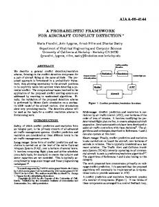
of the specific probability contours that consider the distribution of each IOV in the OVG. The rest of the paper is organized as follows. Section II introduces the details of the proposed multiple vehicle grouping framework. It includes the modeling of the object vehicle group, Bayesian tracking for the IOV states, closeness evaluation, density-based grouping and the OVG state and boundary determination. Section III details numerical experiments that illustrate the workings and the performance of the approach. These include the application of the proposed approach to a real-time traffic intersection scenario in addition to a simulated complex highway scenario involving several vehicles. The potential application of the proposed method to the motion planning of an autonomous vehicle is also discussed in this section. Conclusions are included in Section IV. II. MULTIPLE VEHICLE GROUPING FRAMEWORK The object vehicle grouping framework follows a hierarchical estimation scheme to determine the group structure state G from the state of all detected object vehicles at time k. The overall framework is illustrated in Figure 1. The set denoted by X contains the states and geometrical shapes for all object vehicles. It is obtained by Bayesian IOV tracking given the measurement set Z from sensors. Then, a closeness matrix Mc calculated via probabilistic collision checking between each pair of object vehicles considering uncertainties and their finite geometrical sizes and shapes. Finally, a density-based clustering method (DBSCAN) with a threshold ε is used to group/cluster the IOVs and determine the group structure state G. Each part of the framework is discussed in further detail in the following subsections.

Figure 1 Object vehicle grouping framework

A. Modeling of Object Vehicle Group Assuming there are IOVs indexed from 1 to NOV (NOV>1) that are being tracked at time k, the object vehicle group (OVG) structure state Gk is a collection of labeled vehicle groups:



Gk  G1,k ,..., GNG ,k



(1)

where NG is the number of identified vehicle groups. A vehicle group i is defined as the tuple: Gi ,k  xG ,i ,k , SG ,i ,k , I G ,i ,k , BG ,i ,k , i 1,..., NG ,k 

(2)

3 where xG is the state vector of the group that includes the estimated positions (of a representative point, e.g. centroid) and the velocities of the IOVs in the group as well as their covariances. SG is a parameters set (or generally, an algebraic function fs,G) that may be used to describe the current shape/contour of the group when considered as an extended rigid object. IG is the index set of the IOVs that belongs to the group. All the components of the state vector XG are determined by the states of the IOVs inside the group. BG is the OVG behavior indicating the group structure change from the last time step, which would be one of the following three behaviors: • Behavior 1: Merge. It happens when independent object vehicles or sub-groups merge in to the current group. • Behavior 2: Split. It happens when a group is split into the current sub-group. • Behavior 3: Continue. It happens when the group components stay the same. Therefore, an evolution model of the object vehicle group structure is given by Gk  fG  X k , Gk 1 

(3)

where fG is the grouping function that includes both the closeness evaluation and density-based grouping/clustering, see Figure 1. An example of the evolution of OVG structure is illustrated in Figure 2. Note that an individual group Gi,k will be empty if there are no object vehicles inside it.

Figure 2 Illustration of object vehicle group behaviors (number before dot is vehicle index, number after dot is group index, 0 means no group)

Behavior 1, or, respectively, Behavior 2, are usually activated by the condition that if the calculated probabilistic collision value (after closeness evaluation) between any two IOVs is higher, or respectively lower, than a threshold ε (see the dashed edge connecting the IOVs in Figure 2). The closeness evaluation is introduced in the Section II-C after we discuss the formulation for IOV tracking. B. IOV Tracking For IOV tracking, we apply a Bayesian approach to estimate the motion states and the sizes (by object rigidity assumptions) of all the detected IOVs. By detected IOVs, we mean those falling in the range of the sensing system and deemed of interest for the tracking and guidance problem. Assuming there are

IOVs indexed from 1 to NOV (NOV>1) being tracked at time k, the IOV set X is a collection of labeled IOV tuples:



X k  X 1,k ,..., X NOV ,k



X j ,k  x j ,k , SOV , j ,k , j 1,..., NOV 

(4) (5)

where x is the estimate of the motion state vector of the IOV that includes the positions (a representative point, e.g. centroid) and the velocities of the object vehicle as well as their covariances. SOV is the parameters set (or an algebraic function fs,OV) used to describe the current shape/contour of the object vehicle, e.g. this could be the length and width for a rectangular description or the major and minor length for an elliptical description. Here, we assume SOV and NOV are already identified and we focus on the estimation of the motion state x. Methods to capture SOV, NOV can be found in [7], [8]. The general evolution of the motion state and measurement sequence of an IOV I can be written as: xi ,k  f m,i  xi ,k 1 , wi ,k 1 

(6)

zi ,k  hm,i  xi ,k , vi ,k 

(7)

where fm is a (nonlinear) function of the state x and process disturbance/noise sequence w. z is the available measurement most likely from observation cameras, or on-board distance sensors (lidar). hm is a (possibly nonlinear) function of the states x and measurement noise sequence v. The uncertainties considered in this paper are mainly due to process noise from environmental disturbances like wind, road or un-modeled dynamics acting on the lateral and longitudinal motion of the vehicle and measurement/sensor noise. Later on, we will assume that these uncertainties are captured-well with Gaussian distributions. In the Bayesian approach to tracking the motion state of an IOV i, one attempts to estimate the posterior probability density function (PDF) pi(xi,k|zi,1:k) of the state xi according to all the measurements zi up to time k. Assuming the initial PDF pi(xi,0|zi,0)≡pi(xi,0) is available with no initial measurement z0, then pi(xi,k|zi,1:k) can be obtained by a two-step recursive loop: prediction and update. In the prediction stage, if the required PDF pi(xk-1|z1:k-1) is known, the prior PDF of the state at time k is predicted via the following equation: pi  xi ,k | zi ,1:k 1    pi  xi ,k | xi ,k 1  pi  xi ,k 1 | zi ,1:k 1  dxi

(8)

Note that pi(xi,k|xi,k-1)=pi(xi,k|xi,k-1, zi,1:k-1) is obtained from equation (6) assuming a Markov process and the known statistics of wi,k-1. In the update stage, suppose a measurement zi,k is available, it can be used to correct the prior PDF via Baye’s rule: pi  xi ,k | zi ,1:k  

pi  zi ,k | xi ,k  pi  xi ,k | zi ,1:k 1  pi  zi ,k | zi ,1:k 1 

(9)

Similarly, pi(zi,k|xi,k) is obtained from equation (7) and the known statistics of vi,k. The denominator term pi(zi,k|zi,1:k-1) is given by:

4 pi  zi ,k | zi ,1:k 1    pi  zi ,k | xi ,k  pi  xi ,k | zi ,1:k 1  dxi

(10)

Therefore, by following the recursive loop above, the posterior density of the motion state x for each IOV can be estimated. For a linear description of the motion and measurement system (6) and (7), the analytical solution for the exact posterior PDF can be obtained via the application of Kalman Filter (requiring Gaussian noise v and w,) and Gridbased Estimator (requiring discrete state space). For a nonlinear description of the system (6) and (7), Extended Kalman Filter or Unscented Kalman Filter, Approximate Grid-based Estimator or Particle Filter can be used to approximate the posterior PDF [21]. Without too much loss of generality, hereafter, x represents the motion state (both position and velocity components) for the centroid of the geometric shape of each object vehicle. We will also use x to refer to just the position component of the motion state (e.g. in illustrations), when there is no ambiguity. C. Closeness Evaluation As the state of the IOVs are estimated by the posterior PDF for the centroid of each vehicle (including uncertainty), the Euclidean distance metric is not suitable to represent the closeness between different IOVs. For such a case, the probability of collision between two IOVs can be applied to measure closeness. Let Xi(xi,k) be the state space (position, velocity and shape) occupied by IOV i at time k considering its geometric shape, e.g. an area described by an algebraic function fs,OV,i(x). Then, collision between IOV i and IOV j is defined by the condition C(xi,k, xj,k): Xi,k(xi,k)∩Xj,k(xj,k)≠Ø. Then, the probability of collision between the two IOVs is defined by the integral of the joint state distribution of the IOV i and IOV j: PC  xi ,k , x j ,k     I C  xi ,k , x j ,k  pij  xi ,k , x j ,k dxi dx j

(11)

distributions, an approximate closed-form solution was given in [22] for pairs of small sized objects with one of which can be reduced to a point. Then, the PDF value of the x in X(x) are nearly the same as the one in the centroid of X(x). However, in our case, the sizes of the IOVs are not negligible and such approximations will not work. Therefore, we develop some strategies to approximate the probability of collision between two IOVs with non-negligible geometric sizes and shapes. The first step is to approximate the collision indicator function with a simpler description. Here, we rewrite the definition of the collision condition of two IOVs (with indices i and j) with non-negligible geometric sizes at time k as C’(xi,k, xj,k): xi,k∈Xij,k(xj,k), where Xij,k(xj,k) is an extended deterministic geometric space occupied by IOV j at time k on which we lump the geometric shapes/sizes of both IOVs (with indices i and j). Therein, IOV i is considered as a point. An example of collision in 2D position space between two IOVs with rectangular shapes is shown in Figure 3. One can also similarly derive the extended shape Xij,k(xj,k) for other geometric descriptions like circles or ellipses [19]. Then, the collision condition can be represented by an inequality in terms of the relative distance between xi,k and xj,k. The collision indicator function can be rewritten as:  1, if xi ,k  Xij ,k  x j ,k  I C  xi ,k , x j ,k     0, otherwise

Therefore, (11) can be modified as: PC  xi ,k , x j ,k      p  xi ,k | x j ,k  dxi  p j  x j ,k  dx j (14)  xi ,k Xij ,k  x j ,k  

As the inner integral of (14) constrains the range of xi,k within Xij,k(xj,k), we can define a deviation state variable Δxj,k∈Xij,k(0) to replace xi,k:





xi ,k Xij ,k x j ,k

where IC is the collision indicator function defined by:  1, if Xi ,k  xi ,k  X j ,k  x j ,k   Ø I C  xi ,k , x j ,k     0, otherwise





p  xi ,k | x j ,k  dxi

x j ,k Xij ,k  0 

(12)

This formulation of probability of collision can be implemented via Monte Carlo Simulations (MCS), which are computationally expensive. With assumptions of Gaussian

(13)

p  xi ,k  x j ,k  x j ,k | x j ,k  d x j

(15)

where Xij,k(0) is the lumped space when xj,k is at the origin. Then, PC  xi ,k , x j ,k     p x  x j ,k  x j ,k | x j ,k  d x j  p j  x j ,k  dx j  x j ,k Xij ,k  0  i ,k 

(16)

This integral can be further simplified when the distributions of the states of IOV i and IOV j are Gaussian and independent. Proposition 1: Consider IOV i, with a point description with state xi,k and IOV j with state xj,k and an extended deterministic geometry description Xij,k(xj,k)). If the states xi,k and xj,k have Gaussian distributions, i.e., xi,k~N(mi,k,Σi,k), xj,k~N(mj,k,Σj,k), and the state tracks of IOV i and IOV j are independent, then: PC  xi ,k , x j ,k  



x j ,k Xij ,k  0 

T 1  1  exp    x j ,k  mi ,k  m j ,k   i ,k   j ,k   x j ,k  mi ,k  m j ,k   2  d x

(2 ) nx i ,k   j ,k

j

(17) Figure 3 Example of the collision condition for two IOVs with rectangular shape description in 2D (a is half length and b is half width)

5 where nx is the dimension of the state x (generally comprising of the position and the velocity for each IOV). Poof: Let px(m, Σ) denote the PDF of a multivariate Gaussian distribution for IOV state x. Given the independence assumption: 

  

x j ,k Xij ,k  0 



x j ,k Xij ,k  0 

p  xi ,k  x j ,k  x j ,k | x j ,k  d x j  p  x j ,k  dx j 

 px , j  mi ,k  x j ,k , i ,k  px , j  m j ,k ,  j ,k  dx j  d x j  

(18) Using the fact that the product of two multivariate Gaussian distributions is also a multivariate Gaussian [23]: px , j  mi ,k  x j ,k , i ,k  px , j  m j ,k ,  j ,k   c  px , j  mc,k , c ,k  (19)

where: T 1  1  exp    mi ,k  x j ,k  m j ,k   i ,k   j ,k   mi ,k  x j ,k  m j ,k  2   c (2 ) nx i ,k   j ,k

mc,k   i,1k  j ,1k 

1



1 i ,k

mi ,k  j ,1k m j ,k 

c,k   i,1k  j ,1k 

1

equation (16) may be sought. However, we do not address these cases in this paper. Some discussions in this direction can be found in [22]. Furthermore, for the case of non-Gaussian distributed motion states of IOV i and IOV j, whether these are dependent or not, one may have to resort to MCSs to evaluate the probability of collision directly from (16). Finally, by applying the probabilistic closeness/collision evaluation between each pair of detected IOVs, a closeness matrix 𝑴c can be assembled:  PC  x1,k , x1,k   MC    P x ,x  C NOV ,k 1,k





PC x1,k , x NOV ,k







PC xNOV ,k , xNOV ,k



    

(24)

This matrix will be used in the grouping of IOVs in the next sub-section. (20)

(21) (22)

Using (19)-(22) in equation (18), we have: p  xi ,k  x j ,k  x j ,k | x j ,k  d x j  p j  x j ,k  dx j  (23)  c  px , j  mc ,k , c ,k  dx j ,k  d x j    x j ,k Xij ,k  0   

  

x j ,k Xij ,k  0 

As the inner integral equals to 1, equation (17) is proved. Remark 1: By following the redefinition of the collision condition and Proposition 1, we can see that the problem of evaluating the probability of collision between two IOVs with non-negligible geometric sizes/shapes with Gaussian distributed and independent states can be transformed into one of calculating the integral of a combined multivariate Gaussian density function (defined by equation (20)) within a specified integral space (defined by Xij,k(0)). Furthermore, if the combined covariance Σi,k+Σj,k is diagonal and Xij,k(0) is a combination of closed integral ranges for each variate of Δxj,k, a closed-form solution can be found for the probability of collision by evaluating (17). Remark 2: For evaluation of closeness between IOVs via the collision probability, the state variates are taken from the IOV tracking. The closeness here includes not only the “nearness” in positions but also the “similarities” in velocities between the IOVs. Similar to the rectangles used to illustrate the closeness in positons (in Figure 3 and discussions above), a speed range can also be used to define the closeness in velocities. With x interpreted as the motion state vector (position and velocity), both aspects of closeness are already considered above, including in the specification of the integral space Xij,k(0). Only if the nearness in both positions and velocities are satisfied are any two IOVs considered close to each other. If the Gaussian distributed motion states of IOV i and IOV j are dependent as is possible for cases with mutual interactions, a different result that approximates the collision probability

D. Density-Based Grouping/Clustering Here, we adopt the Density-based Spatial Clustering of Applications with Noise (DBSCAN) approach [24] to group the detected IOVs by processing the closeness matrix given by equation (24). The probability of collision (value between 0 and 1) between the pairs of IOVs provides a good one-dimensional closeness indicator that be used with DBSCAN [25]. DBSCAN is widely applied in machine learning and data mining for clustering purposes due to its attractive attributes: • The number of clusters/groups in the data set is not required to be pre-specified. • Only two parameters are required: the closeness threshold ε in the neighborhood of any object i and the minimum number of other objects μ that are within the threshold ε of object i. • It is suitable for arbitrarily shaped clusters/groups. The key idea we adopt from this approach for vehicle grouping is that for the main object components of an OVG, at least a minimum number μ of IOVs should be contained in the neighborhood of a given closeness threshold ε (between 0% and 100%). Here, we emphasize that selecting an appropriate ε is very important as it’s directly related to the success of the grouping algorithm. For example, a too small ε (≈0%) may lead to big groups with low-closeness IOVs inside, and a too large ε (≈0%) may fail in grouping the IOVs even for those with high closeness. A proper range for ε could depend on the situation (urban, highway, intersection, etc). Here, we select ε to be 0.5 (average of the collision probability of 0% and 100%) for our

Figure 4 Illustration of the DBSCAN grouping results (μ=4). The edge means there is density-connection between the IOVs. Only the group index of each IOV is shown here. 0 means the IOV is SOV with no group index.

6 illustrations. The selection of μ depends on the density of the objects. These main object components in the group are defined as core object vehicles (COVs). The closeness threshold ε defines a density connection condition between two IOVs: if PC(xi,k, xj,k)≥ε, IOV i and IOV j are said to be density connected with each other. There can also be another kind of IOV called border object vehicle (BOV) in the group that can’t satisfy the minimum number μ requirement for being a COV but can be connected with COVs. In addition, there can be IOVs not connected with any COVs. These are considered as single object vehicles (SOVs). An illustration of these different kinds of objects is given in Figure 4. The algorithm is detailed in [24]. Once the clustering/grouping is done, each IOV will be labeled with its updated OVG index from 0 to NG. And all the indices of the IOVs in OVG i will be stored in an index set as IG,i. Furthermore, the group behavior BG,i can also be determined by evaluating the OVG index for each IOV at sequential time steps. Although the DBSCAN approach is only applied here to identify the OVGs and label the IOVs with their OVG index, the motion state for OVG i xG,i at time k can be obtained from the mixed state distribution of those IOVs in the group: xG ,i ,k 

N IG ,i ,k



G ,i , j , k

j 1

p

I G ,i ,k ( j )

x

I G ,i ,k ( j ), k

dx

I G ,i ,k ( j )

calculation, we obtain a conservative evaluation of the collision probability:

PG ,i  xk  

N IG ,i ,k

 P x  j 1

j

k

(30)

We say equation (30) is a conservative evaluation because the probability is overestimated by simply adding the probabilities based on the distribution of each IVO. This is known as the Boole’s inequality or union bound [26]:   N IG ,i ,k P x j ,k  xk    Pj  xk   jI  j 1  G , j ,k 

(31)

The OVG boundary is then obtained by drawing the probability contour using numerical methods: N IG ,i ,k      xk :  Pj  xk    , 0    1 j  1    

(32)

A comparison of the OVG boundaries determined by equation (29) and (30) is illustrated in the example in Figure 5. We can see the probability of the group distribution is bounded by (30).

(25)

where NIG,i,k is the number of elements in the index set IG,i at time k. The weights for different IOV distributions can be determined based on the closeness of each IOV to other IOVs in the same OVG:  j ,k 



iI G ,i ,k \ I G ,i ,k  j  N IG ,i ,k







PC xIG ,i ,k ( j ),k , xi ,k

j 1 iI G ,i ,k \ I G ,i ,k  j 





PC xIG ,i ,k ( j ),k , xi ,k

(26)



Finally, the shape of the OVG i at time k can be described by the boundary of an area with a specified joint probability distribution among all the IOVs in the OVG i, i.e. the set:

x

: PG ,i  xk    , 0    1

(27)

  PG ,i  xk   P  x j ,k  xk   jI   G ,i ,k 

(28)

k

According to the inclusion-exclusion principle of set theory, equation (28) becomes:   N IG ,i ,k   P x j ,k  xk    Pj  xk    P  x j ,k  xk   jI  j 1 J  I G ,i ,k  jJ   G , j ,k  J 2     N +  P  x j ,k  xk     ( 1) IG ,i ,k P  x j , k  xk   jI  J  I G ,i ,k  jJ   G ,i ,k  J 3

Figure 6 Illustration of the OVG distribution contour in a 2D position space. The position states of the three IOVs are assumed to be Gaussian distributed. a=0.1 and a=0.9 contours shown. Solid probability contours are calculated by (29) while the dash contours come from (30).

III. NUMERICAL EXPERIMENT To illustrate the performance of the proposed object vehicle grouping framework, we first include the setup and results of a numerical experiment that represents a complex highway scenario. Several methods are compared for use in the closeness evaluation and the salient aspects of the group tracking approach are illustrated with this scenario. We then present the results of the application of the proposed approach to a real-

(29)

As calculating the intersection distribution probability among the IOVs in the OVG requires multiple integrals (with the order equal to the number of IOVs in the group), it’s hard to evaluate the probability of collision via equation (29), especially when NIG,i,k had a large value. Therefore, we need a tractable approximation to (29). If we ignore the intersection probability

Figure 5. Particle motion description for the IOV

7 time traffic intersection scenario from the Next Generation Simulation (NGSIM) project database available on the Research Data Exchange of the U.S. Department of Transportation’s Federal Highway Administration [27]. In both scenarios, we assume a centralized surveillance view of the IOVs from the ego-vehicle or roadside infrastructure, and illustrate the performance of the vehicle grouping algorithm. A. Complex Highway Scenario 1) Simulation Settings In the highway scenario, we use a kinematic particle motion model defined in the Frenet frame for IOV state tracking purposes. See Figure 6 for the important notations and the coordinate frame. This model has been used in our previous works [28], [29] for motion planning purposes. The reference path is define by its curvature κ(s) as a function of the arc length s. We assume the reference path is already known and the IOVs are going to follow it (with their respective controlled dynamics that describe forward motion like cruising or acceleration and lateral motion like lane change). One possible description of the controlled dynamics of the IOVs is: 1 0 0  0  so     so   v s   0  K s1   vts,o  0 0  t ,o    1  K s 2    y e ,o     y e ,o  0 0 1  s   s  0 v  v n ,o   0   n ,o  0  K  K y1 y2   0  0  0  0  K   1  s1  0   vts,o ,ref   0  ws ,o  (33) 1  K s 2     1  K s 2  w    ye ,o ,ref   y , o  0  0   0  0  0  0 K y1  1   so   yso  1 0 0 0  vts,o  1 0  vs ,o        y   0 1  v  y 0 0 1 0 e , o     y ,o   ye ,o    s  v  n ,o  where, so and ye,o are, respectively, the arc length and lateral position error of the IOV; vts,o and vns ,o are, respectively, the

Figure 7 Geometric shape of the IOV i in the numerical simulation (cs is a constant time gap to adjust the safety margin)

calculate the closeness in positions, the geometric shape of the IOV is defined as a rectangle with a car-like realistic size (a for half length and b for half width). Also, in the numerical experiment, we will add a safety margin csvst,o,i that is related to the velocity of the IOV i in its geometric length to mimic human-driver like actions that keep a safe distance between a front and rear vehicle, as shown in Figure 7. For the closeness in velocity, we define a bound [-Δvt, Δvt] for the velocity difference between two IOVs. This will factor in following and leading conditions in the probabilistic inclusion/exclusion of IOVs in groups. After the closeness evaluation, the OVGs will be identified via DBSCAN w.r.t the closeness threshold ε and the minimum number μ. Here we choose μ=2 due to the small numbers of IOVs (low density) in the present example, which considers 8 IOVs on a highway scenario (described below). Therefore, in this case, the BOV and COV are the same. All the parameters used in the numerical experiment are given in Table I. TABLE I. Parameters of IOVs in the numerical experiment Parameter ws ,o [m/s]

Value

Parameter

Value

Parameter

Value

N(0,25)

Ks2

2

cs [s]

0.5

N(0,1)

K y1

2.5

Δvt [m/s]

1

vs ,o [m]

N(0,25)

K y2

2

ε

0.5

v y ,o [m]

N(0,1)

a [m]

3.75

μ

2

K s1

2.5

b [m]

1.6

α

0.5

w y ,o

[m]

tangential speed and normal speed of the IOV along their reference path. Ky1 and Ky2 are the proportional and integral gains of a controlled OV tracking its reference lane ye,o,ref. Ks1 and Ks2 are the proportional and integral gains of a controlled OV tracking the reference speed vts,o,ref . We assume that ws ,o and wy ,o are Gaussian disturbances perturbing the input references vts,o,ref

and ye,o,ref; and vs ,o

and v y ,o

are the Gaussian

measurement noises on sensors for so and ye,o. Here, we assume that the measurements are obtained without sensor delay, faults or sensing range limitations. With such linear dynamics models for the IOVs, a regular KF can be used to estimate the states of the IOVs. Note that even more refined implementations such as Interactive Multi-Model KF [30] and higher order models are also possible to use for IOV state estimation and integrated with our grouping function/approach as depicted in Figure 1. As for the closeness calculation, we consider both the closeness in positions and velocity in the two scenarios. To

Figure 8 States of the IOVs in a highway scenario. Top: relative positions, Bottom longitudinal velocities.

8 The highway scenario we constructed is a sequence of typical highway situations, like cruising, overtaking, following etc, are specifically selected to illustrate the nuances of the group evolution for a span of 90 seconds. The reader is encouraged to look at the state tracking (estimation) results for all IOVs shown in Figure 8 at this point. These are elaborated further in the next subsection. We compare our proposed approach to closeness evaluation and grouping in the highway scenario, we compare our numerical integration (NI) method on the derived condition (17) with the Monte Carlo Simulations (MCS) using 100000 samples (can approximate a probability accuracy up to 0.001%). We also consider the approximation method for small sized objects (ASO) proposed in [22] and described earlier. In ASO, the collision probability is evaluated by: PC  xi ,k , x j ,k   T 1  1  exp    x j ,k  mi ,k  m j ,k   i ,k   j ,k   x j ,k  mi ,k  m j ,k   2   Vs (2 ) nx i ,k   j ,k

(34)

where Vs is the volume of Xij,k(0). 2) Results and Discussions First, we start with a comparison of the closeness evaluation methods. When applying NI and MSC (with 100000 samples) in closeness evaluation, the same group structure evolution profile is obtained (see Figure 9). However, no group structure evolution is found in the ASO case (not plotted here); with ASO, the group index of all IOVs remain at 0 as individuals. These can be explained by the evaluated closeness profiles between each pair of IOVs under the three methods, as shown in Figure 10 and Figure 11, herein, the closeness evaluated by NI and MSC are almost the same (with accuracy up to 0.001%). In addition, the RMS of the errors between the closeness evaluation using MSC with different samples and NI, ASO and NI for the IOVs shown in Figure 10 and Figure 11 are given in Table II. As more samples are used, the error between the closeness evaluation MSC and NI become smaller, which demonstrate the validity of our NI method. However, for ASO,

Figure 9 Closeness between IOV 3 and some of the other IOVs under the Monte Carlo Simulation(MSC) method with 100000 samples, numerical integration (NI) method, and the approximation method for small-sized object (ASO).

Figure 11 Closeness between IOV1 and some of other IOVs under the three methods

Figure 10 Group structure evolution for the highway scenario with application of either the NI or MSC methods for closeness evaluation.

the closeness is always 0 and the RMS error between NI and ASO is large. This is due to the fact that the size of the IOV is too large compared with the distribution area covered by the uncertainties. From (34), it’s obvious that ASO uses the probability density value at the center of Xij,k(0) to represent the density value for the other locations in Xij,k(0). This only works when the size of object, i.e. the volume of Xij,k(0), is small. Otherwise, we obtain zero density value when the two objects are too far away relative to the distribution area arising from the uncertainties. Therefore, ASO is not suitable to use in cases with non-negligible geometric sizes of the objects involved (i. e, real highway vehicles). The computational time for evaluating the closeness between a pair of IOVs under the three methods are also summarized in Table III (on a notebook PC with Intel i5-4200M

9 2.4 GHz processor and 4GB RAM). ASO is most efficient, but as described above is least accurate. The proposed NI gives a reasonably efficient resolution of the closeness evaluation when a high accuracy of probability evaluation, e.g. smaller than 0.01%, should be ensured. MSC is most accurate but is unlikely to be useable for real-time applications. TABLE II. RMS of the error between other methods and NI in evaluating the closeness of two IOVs shown in Figure 10 and Figure 11.

RMS Error IOV3 and IOV 1 IOV3 and IOV4 IOV3 and IOV5 IOV3 and IOV6 IOV1 and IOV2 IOV1 and IOV6 IOV1 and IOV7

MCS (100000 samples) 0.00018 0.00033 0.00030 0.00027 0.00041 5.52e-6 7.61e-6

Method MCS (10000 samples) 0.0005 0.0012 0.0010 0.0009 0.0013 1.79e-5 2.30e-5

MCS (1000 samples) 0.0014 0.0034 0.0030 0.0030 0.0039 6.01e-5 7.46e-5

ASO 0.1848 0.4402 0.7173 0.7163 0.664 1.02e-5 1.75e-5

2 splits into SOV 1 and SOV 2 at t=74s. However, IOV 2 moves laterally towards the lane occupied by IOV 1. To avoid a collision, IOV 1 decelerates and change lane to the right. When IOV 2 settles down, IVO 1 accelerates to overtake it. During this collision avoidance process, we can see the oscillation of the closeness value between IOV 1 and IOV 2 in Figure 11Error! Reference source not found. between t=74~85s. This is mainly due to the rapid velocity change of IOV 1 to avoid a collision and then overtake the slower IOV 2. We can also generate the group geometry description for this scenario. Figure 12 shows an example for the position description sampled at time t=15 and 60s. Here, we use a belief contour with α=0.5 to represent the distribution of the OVGs. The OVG position center calculated by applying equations (25) is also shown. Each IOV is labeled with their group index behind their IOV index. We can see how the group boundary contour and center position changes along with the indices of the IOVs in the OVG from t=15 to 60s, as shown in Figure 12.

TABLE III. Execution time of the error in evaluating the closeness of two IOVs for 3168 runs under different methods on a notebook with Intel i54200M 2.4 GHz processor and 4GB RAM. Execution Time Max [ms] Min [ms] Mean [ms]

MCS (100000 samples) 33.9 11.5 11.7

Method MCS MCS (10000 (1000 samples) samples) 1.16 0.232 0.634 0.116 0.717 0.123

NI

ASO

0.762 0.483 0.495

0.036 0.018 0.019

In Figure 9, we can see the total number of OVGs identified evolves as 2-1-2-1-2-3-2-3-2-3-2, as the states for the IOVs evolve differently. Initially, IOVs 1, 2, 5 and 6 are all SOVs as they are far away from other IOVs in positions. IOV 1 and IOV 2 are also different form other IOVs in velocity, see Figure 8. While IOVs 3, 4 are grouped in OVG 1 (see Figure 10 for the closeness values) and IOV 7, 8 are in OVG 2 due to their closeness both in positions and velocity. As time goes, SOV1 changes lane to overtake IOV 3, 4 around t=10s and then IOV 3 starts to accelerate and move towards SOV 5 and SOV 6. As a result, OVG 1 splits into SOV 3 and SOV 4 around t= 20s, and OVG 2 becomes OVG 1. During the acceleration, SOV 3 is caught up by SOV 1 and they temporally merge into the new OVG 1 at t=27s. As IOV 1 tries to keep its fast speed, it decides to change lane to follow the faster IOV 2 among the rest of the IOVs to pass through the traffic jam formed by IOVs 5, 6, 7 and 8 (The details of the motion control decisions are discussed in our other work [29]). Therefore, the OVG 1 split again at t=31s and SOV 1 and 2 merge into the new OVG 1 at t=33s, see Figure 11. Later SOV 3 decelerate to merge with SOV 5 and SOV 6 to form a new OVG 2 at t=45s. When a faster IOV passes by a slower IOV through an adjacent lane, we can see the rise of closeness between them, for example, the closeness of IOV 1 and 6 and IOV 1 and 7 rises when IOV1 is passing through the traffic jam as can be seen in Figure 11. However, as can be seen in Figure 8, the longitudinal velocity gap between them is too large (two times larger than the specified bound of the velocity difference Δvt) to significantly increase the closeness. After IOV1 pass through the traffic jam together with IOV 2 in OVG 2, it changes lane to overtake IOV 2 and then OVG

(a)

t=15s

(b)

t=60s

Figure 12 Example of relative position description of OVGs at different time for highway scenario. See Figure 2 for adopted numbering convention.

B. Application to Real-Time Traffic Intersection Data Set For simplicity and to avoid duplication, in the intersection scenario, we only apply our grouping function with the NI method of closeness evaluation. We apply the grouping function to the vehicle trajectory data generated by the NGVIDEO software after processing a 15 min overhead camera record of actual traffic in an intersection on Lankershim Boulevard in Los Angeles, CA (data from [27]). Here, we chose one segment from t = 5min23s to 5min52 to show the typical vehicle grouping results as an example. The position description of the OVGs are sampled at 6 frames, as shown in Figure 13. We can clearly see the group formation (OVG1) of a set of IOVs (IOV2~IOV6) from SOVs at t = 5min23s to a unique group at t = 5 min 42 (Figure 13 (a)~(c)) when these IOVs stop before a red light. The closeness profile between the front and rear IOVs in this case are not given here, but it’s similar to the case of IOV 3 and IOV5 or IOV6 in the highway

10

(a) t=5min23s

(b) t=5min26s

(c) t=5min42s

(d) t=5min44s

(e) t=5min48s

(f) t=5min52s

Figure 13 Example of position description of OVGs at different time for the intersection scenario under NI method in closeness evaluation. See Figure 2 for the adopted numbering convention.

scenario above with velocity synchronization (0 m/s) and position proximity at the end. Then, more and more IOVs slow down to approach OVG1 with different velocities from behind. Among these IOVs, the ones with similar velocities and close distance merge into groups, as shown in the group identities in Figure 13 (c)~(e). After IOV1 completes its left turn, the light turns green, and the set of IOVs start to pass the intersection with some distinct or some similar accelerations, therefore, big OVGs split into small OVGs, as shown in Figure 13 (f). We can see the grouping method successfully identifies the IOVs with common and distinct motion and accordingly adjusts the group identities in this intersection scenario. C. Comments on the Application of Grouping to Motion Planning for Autonomous Vehicles As the group boundary represents the probability of the distribution of the IOVs in the OVG, it can be used to re-define the multitude of obstacle avoidance constraints that arise in the real-time motion planning of autonomous vehicles in uncertain public traffic involving many vehicles. Such planning

frameworks were discussed, for example, our previous works [28], [29] that discuss predictive control approaches and even those of [31]that use rapidly exploring random trees. In this paper, we considered probabilistic collision problems involving IOVs with non-negligible geometric shapes and derived the condition given in equation (16) and given a simplified derivation in Proposition 1 for the case of Gaussian distribution of the motion states. If we only apply the chanced constraints derived from these results for collision avoidance of the Autonomously Controlled Vehicle (ACV or ego-vehicle) with each detected IOV, in the numerical optimization problem of predictive motion planning, some undesirable local minimums will result the intersections of the collision boundaries of IOVs (with some closeness) that will trap the ACV from finding better solutions for its motion plan. We have shown earlier that for deterministic planning [19] [20], a good OVG algorithm can help to tailor the feasible field to exclude these effects. In principle, one can expect this to work for the probabilistic planning case as well since the chanced constraints (representing avoidance of IOVs and OVGs) can be

11 numerically transformed to the deterministic constraints for the optimization problem to find a solution [32]. However, the real-time motion planning problem requires a real-time solution of the group boundary generation, like the ASO method. To determine the group contours for the illustrations in this paper, we used numerical methods (integrations or simplified solution mentioned in Remark 1) to sample a set of points based on the collision probability evaluation. While this represents the true boundary, its computation may not be efficient for real-time implementation in all scenarios. Therefore, in our continuing work, we approximate the probabilistic collision condition and the contour of the OVGs with conservative closed-form results, similar as the OVG boundary for the deterministic case in [19] [20], and apply it in stochastic motion planning algorithms for autonomous vehicles. IV. CONCLUSION In this paper, we propose a probabilistic multiple vehicle grouping framework for tracking the evolution of groups of individual object vehicles (IOVs) with the consideration of their non-negligible geometric sizes and prevalent sensing and motion uncertainties. Therein, the closeness between any two IOVs, which is defined by a probabilistic collision condition comprising of mutual proximity both in velocities and positions as the main criteria for subsequent clustering of detected vehicles into object vehicle groups (OVGs) whose states are estimated by the weighted distribution of each IOV in the OVG. The workings and performance of our proposed framework are illustrated for a simulated complex scenario and a real-time traffic intersection dataset. Comparison of the probabilistic collision condition as derived and evaluated via a numerical integration method with Monte Carlo Simulations show that it can achieve very good accuracy with about a 20x computational speed up. It is also highlighted that while computationally more efficient approaches of closeness evaluation that ignore geometric sizes exist, they could not resolve group attributes and are not applicable for road vehicles. Continuing work focuses on finding better approximations of the closeness evaluation to further reduce its computational complexity and on determining the OVG boundary so that it can be executed in real-time within stochastic motion planning algorithms for autonomous vehicles. Other aspects that need to be addressed (where the approach may fail) include analysis of other types of uncertainty that could not be modeled as Gaussian, such as most sensor range/view limitations, delays, faults and clutter.

Carlo methods," IEEE Transactions on Signal Processing, vol. 59, no. 4, pp. 1383-1396, 2011. [4]

S. K. Pang, J. Li and S. J. Godsill, "Detection and tracking of coordinated groups," IEEE Transactions on Aerospace and Electronic Systems , vol. 47, no. 1, pp. 472-502, 2011.

[5]

N. Petrov, L. Mihaylova, A. Gning and D. Angelova, "A novel sequential Monte Carlo approach for extended object tracking based on border parameterisation," in In Information Fusion (FUSION), 2011 IEEE Proceedings of the 14th International Conference on, 2011.

[6]

B. Ristic and D. Salmond, "A study of a nonlinear filtering problem for tracking an extended target," in 2004 IEEE Seventh International Conference on Information Fusion, 2004.

[7]

K. Granström, C. Lundquist and U. Orguner, "Tracking rectangular and elliptical extended targets using laser measurements," in Information Fusion (FUSION), 2011 IEEE Proceedings of the 14th International Conference on, 2011.

[8]

K. Granström, S. Reuter, D. Meissner and A. Scheel, "A multiple model PHD approach to tracking of cars under an assumed rectangular shape," in Information Fusion (FUSION), 2014 17th IEEE International Conference on , 2014.

[9]

M. Baum and U. D. Hanebeck., "Shape tracking of extended objects and group targets with star-convex RHMs," in Information Fusion (FUSION), 2011 IEEE Proceedings of the 14th International Conference on, 2011.

[10]

J. Lan and X. R. Li, "Tracking of extended object or target group using random matrix—part II: irregular object," in In Information Fusion (FUSION), 2012 IEEE 15th International Conference on, 2012.

[11]

D. Reid, "An algorithm for tracking multiple targets," IEEE transactions on Automatic Control, vol. 24, no. 6, pp. 843-854, 1976.

[12]

P. Willett, Y. Ruan and R. Streit, "PMHT: problems and some solutions," IEEE Transactions on Aerospace and Electronic Systems, vol. 38, no. 3, pp. 738-754, 2002.

[13]

B. Vo and W. Ma, "The Gaussian mixture probability hypothesis density filter," IEEE Transactions on signal processing, vol. 54, no. 11, pp. 4091-4104, 2006.

[14]

Y. Bar-Shalom and E. Tse, "Tracking in a cluttered environment with probabilistic data association," Automatica, vol. 11, no. 5, p. 451–460, 1975.

[15]

B.-N. Vo, S. Singh and A. Doucet, "Sequential Monte Carlo methods for multitarget filtering with random finite sets," IEEE Transactions on Aerospace and electronic systems, vol. 41, no. 4, pp. 1224-1245, 2005.

[16]

S. Wender and K. Dietmayer, "3D vehicle detection using a laser scanner and a video camera," IET Intelligent Transport Systems, vol. 2, no. 2, pp. 105-112, 2008.

[17]

A. Petrovskaya and S. Thrun, "Model based vehicle detection and tracking for autonomous urban driving," Autonomous Robots, vol. 26, no. 2-3, pp. 123-139, 2009.

[18]

T. Chen, T. B. Schon, H. Ohlsson and L. Ljung, "Decentralized particle filter with arbitrary state decomposition," IEEE Transactions on Signal Processing, vol. 59, no. 2, pp. 465-478, 2011.

[19]

Q. Wang and B. Ayalew, "Obstacle Filtering Algorithm for Control of an Autonomous Road Vehicle in Public Highway Traffic," in Proceedings of the ASME 2016 Dynamic System and Control Conference (DSCC), Minneapolis, MN., 2016.

[20]

Q. Wang and B. Ayalew, "A multiple vehicle group modelling and computation framework for guidance of an autonomous road vehicle," in Proccedings of the 2017 American Control Conference, 2017.

[21]

M. Arulampalam, S. Maskell, N. Gordon and T. Clapp, "A tutorial on particle filters for online nonlinear/non-Gaussian Bayesian tracking," IEEE Transactions on signal processing, vol. 50, no. 2, pp. 174-188, 2002.

[22]

N. E. Du Toit and J. W. Burdick, "Probabilistic collision checking with chance constraints," IEEE Transactions on Robotics, vol. 27, no. 4, pp. 809-815, 2011.

[23]

K. B. Petersen and M. S. Pedersen, "The matrix cookbook," 2008. [Online]. Available: http://www2.imm.dtu.dk/pubdb/views/edoc_download.php/3274/pdf/i mm3274.pdf.

REFERENCES [1]

L. Mihaylova, A. Y. Carmi, F. Septier, A. Gning, S. K. Pang and S. Godsill, "Overview of Bayesian sequential Monte Carlo methods for group and extended object tracking," Digital Signal Processin, vol. 25, pp. 1-16, 2014.

[2]

K. Granstrom and M. Baum, "Extended object tracking: introduction, overview and applications," 2016. [Online]. Available: https://arxiv.org/abs/1604.00970.

[3]

A. Gning, L. Mihaylova, S. Maskell, S. K. Pang and S. Godsill, "Group object structure and state estimation with evolving networks and Monte

12 [24]

M. Ester, H.-P. Kriegel, J. Sander and X. Xu, "A density-based algorithm for discovering clusters in large spatial databases with noise," in Proceedings of the Second International Conference on Knowledge Discovery and Data Mining (KDD-96), 1996.

[25]

H.-P. Kriegel and M. Pfeifle, "Density-based clustering of uncertain data," in In Proceedings of the eleventh ACM SIGKDD international conference on Knowledge discovery in data mining, 2005.

[26]

A. F. Karr, Probability, New York: Springer-Verlag, 1993.

[27]

"NGSIM Program Database," FHWA, 2016. [Online]. Available: https://www.its-rde.net/index.php/rdedataenvironment/10023.

[28]

T. Weiskircher, Q. Wang and B. Ayalew, "A Predictive Guidance and Control Framework for (Semi-)Autonomous Vehicles in Public Traffic," IEEE Transactions on Control Systems Technology, vol. PP, no. 99, pp. 1-13, 2017.

[29]

Q. Wang, B. Ayalew and T. Weiskircher, "Predictive Maneuver Planning for an Autonomous Vehicle in Uncertain Public Traffic,"

Qian Wang received his diploma and master degree in vehicle engineering from the South China University of Technology, Guangzhou, China in 2010 and 2013. Since May 2014, he has been a PhD candidate with the Applied Dynamics and Control Research Group at Clemson University, USA. His research interests include optimal control, predictive trajectory planning for autonomous vehicles, and control allocation for vehicle actuation system.

Dr. Beshah Ayalew is Professor of Automotive Engineering and director of the DOE GATE Center of Excellence in Sustainable Vehicle Systems at Clemson University. He received his MS (2000) and Ph.D. (2005) degrees in Mechanical Engineering from Penn State University. His interest and expertise is in systems dynamics and controls. Dr. Ayalew received the Ralph Teetor Educational Award from SAE (2014), the Clemson University Board of Trustees Award for Faculty Excellence (2012) and the NSF CAREER Award (2011). He was a recipient of the Penn State Alumni Association Dissertation Award (2005). He is an active member of ASME’s Vehicle Design Committee, IEEE’s Control Systems Society, and SAE.

IEEE Transaction on Intelligent Vehicles, Vols. (Submitted, in review), 2016. [30]

E. Mazor, A. Averbuch, Y. Bar-Shalom and J. Dayan, "Interacting multiple model methods in target tracking: a survey," IEEE transactions on aerospace and electronic systems, vol. 34, no. 1, pp. 103-123, 1998.

[31]

Y. Kuwata, J. Teo, G. Fiore, S. Karaman, E. Frazzoli and J. P. How, "Real-time motion planning with applications to autonomous urban driving," IEEE Transactions on Control Systems Technology, vol. 17, no. 5, pp. 1105-1118, 2009.

[32]

S. A. Tarim, S. Manandhar and T. Walsh, "Stochastic constraint programming: A scenario-based approach," Constraints, vol. 11, no. 1, pp. 53-80, 2006.