A Probabilistic Graphical Model for Recognizing NP ...

A Probabilistic Graphical Model for Recognizing NP Chunks in Texts Minhua Huang and Robert M. Haralick Computer Science, Graduate Center City University of New York New York, NY 10016 [email protected] [email protected]

Abstract. We present a probabilistic graphical model for identifying noun phrase patterns in texts. This model is derived from mathematical processes under two reasonable conditional independence assumptions with different perspectives compared with other graphical models, such as CRFs or MEMMs. Empirical results shown our model is effective. Experiments on WSJ data from the Penn Treebank, our method achieves an average of precision 97.7% and an average of recall 98.7%. Further experiments on the CoNLL-2000 shared task data set show our method achieves the best performance compared to competing methods that other researchers have published on this data set. Our average precision is 95.15% and an average recall is 96.05%. Key words: NP chunking, graphical models, cliques, separators

1

Introduction

Noun phrase recognition, also called noun phrase chunking (NP chunking), is a procedure for identifying noun phrases (NP chunks) in a sentence. These NP chunks are not overlapping and not recursive [1]; that is, they can not be included in other chunks. Although the concept of NP chunking was first introduced by [1] for building a parse tree of a sentence, these NP chunks provide useful information for NLP tasks such as semantic role labeling or word sense disambiguation. For example, a verb’s semantic arguments can be derived from NP phrases and features with syntactic and semantic relations for word sense disambiguation can be extracted from NP phrases. The methods for classifying NP chunks in sentences have been developed by [2], [3], [4], [5]. Of the methods reported, the best precision is 94.46% and the best recall is 94.60% on the CoNLL-2000 data. In this paper, we discuss a new method for identifying NP chunks in texts. First, a probabilistic graphical model is built from different perspectives compared with other existed graphical models under two conditional independence assumptions. Moreover, the corresponding mathematical representation of the model is formed. Finally, decision rules are created to assign each word in a sentence to a category (class) with a minimal error. As a consequence, a sentence is

attributed to a sequence of categories with the best description. Finally, grouping consecutive words of the sentence with the same assigned specific classes forms a NP chunk. In experiments on the Penn Treebank WSJ data, our method achieves a very promising result: the average recall is 97.7%, the average of precision is 98.7% and the average of f-measure is 98.2%. Moreover, in experiments on the CoNLL2000 data, our methods does better than any of the competing techniques: the average recall is 95.24%, the average precision is 96.32%, and the f-measure is 95.83%. The rest of the paper is structured in the following way. The second section presents the proposed method. The third section demonstrates the empirical results. The fourth section reviews related researches. The fifth section gives a conclusion.

2 2.1

The Proposed Method An Example

Table 1 shows that an input sentence with it POS tags. Then, by our method, it is assigned to three different categories. Finally, NP chunks are derived from these categories.

Table 1. An example NP chunking procedures Word The doctor was among dozens of people miling through East Berline ’s Gethsemane Church Saturday morning

POS Category NP chunks Number of chunks √ DT C1 1 √ NN C1 VBD C2 IN C2 √ NNS C1 2 IN C2 √ NN C1 3 VBG C2 IN C2 √ NNP C1 4 √ NNP C1 √ POS C3 5 √ NNP C1 √ NNP C1 √ NNP C3 6 √ NN C1

2.2

Describing the Task

Let U be a language, V be vocabulary of U , and T be P OS tags of V . Let S be a sequence of symbols associated with a sentence, S = (s1 , ..., si , ..., sN ), si =< wi , ti >, wi ∈ V, ti ∈ T . Let C be a set of categories, C = {C1 , C2 , C3 }, where C1 indicates the current symbol is in an NP chunk, C2 indicates the current symbol is not in an NP chunk, and C3 starts a new NP chunk. The tasks can be stated as follows: Given S = (s1 , ..., sN ), we need 1. to find a sequence of categories, (c1 , ..., cN ), ci ∈ C, with the best description of S; 2. to determine NP chunks based on (c1 , ...cN ). 2.3

Building Probabilistic Graphical Models

Given S = (s1 , s2 , ..., sN ), C = {C1 , C2 , C3 }, for si ∈ S, we want to find ci ∈ C, s.t. (c1 , c2 , ..., cN ) = argmax p(c1 , c2 , ..., cN |s1 , s2 , ..., sN ) c1 ,c2 ,...,cN

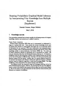
p(c1 , c2 , ..., cN |s1 , s2 , ..., sN ) = p(c1 |c2 , ..., cN , s1 , s2 , ..., sN ) × p(c2 |c3 , ..., cN , s1 , s2 , ..., sN ) × .... × p(cN |s1 , s2 ..., sN ) Suppose ci is independent of cj6=i given (s1 , s2 , ..., sN ). Then, p(c1 , ..., cN |s1 , ..., sN ) can be represented as Fig 1.

Fig. 1. The graphical model of p(c1 , ..., cN |s1 , ..., sN ) under the assumption ci is independent of cj6=i given (s1 , s2 , ..., sN ).

Based the assumption we have made, p(c1 , c2 , ..., cN |s1 , s2 , ..., sN ) =

N Y i=1

p(ci |s1 , ..., sN )

(1)

Assume ci is independent of (s1 , .., si−2 , si+2 , .., sN ) given (si−1 , si , si+1 ) p(c1 , c2 , ..., cN |s1 , s2 , ..., sN ) =

N Y

p(ci |si−1 , si , si+1 )

(2)

i=1

A probability graphical model for p(c1 , ..., cN |s1 , ..., sN ) is constructed. Fig 2 shows this model. From this model, a set of N + 1 cliques1 is obtained: CIL = {p(s1 , s2 , c1 ), p(s1 , s2 , c2 ), ..., p(sN −1 , sN , cN ), p(sN −1 , sN , cN )} Moreover, a set of 2N − 3 separators

2

is received:

SEP = {p(s1 , s2 ), ..., p(sN −1 , sN ), p(s2 , c2 ), ..., p(sN −1 , cN −1 )}. From this model, according to [6], p(c1 , .., cN |s1 , .., sN ) can be computed by the product of cliques divided by the product of separators.

Fig. 2. The probabilistic graphical model of p(ci |s1 , ...sN ) under assumptions ci is independent of cj6=i given (s1 , s2 , ..., sN ) and ci is independent of (s1 , .., si−2 , si+2 , .., sN ) given (si−1 , si , si+1 )

Hence: p(c1 , ..., cN |s1 , ..., sN ) ∝

N Y

p(si−1 |si , ci )p(si+1 |si , ci )p(si |ci )p(ci )

(3)

i=1

Differences between Other Graphical Models. What is the different between our model and other graphical models? In Fig 3, we show a HMM[7], a second order HMM[4], a MEMM[7], a CRF[8], and the model of us. For simplicity, we just show the si part. These models represent a joint probability p(s1 , ..., sN , c1 , ..., cN ) or a conditional probability p(c1 , ..., cN |s1 , ..., sN ) under 1 2

a clique is a maximal complete set of nodes. Γ = {Γ1 , ..., ΓM } is a set of separators, where Γk = Λk ∩ (Λ1 ∪ ..., ∪Λk−1 ).

different conditional independence assumptions. By observing these models, the structure of our model is different from other models. From empirical results on CoNLL-2000 shared task data set, our model can achieve the better performance than HMMs. However, there are no comparisons between our model with M EM M s or CRF s.

QN Fig. 3. (1): a HMM model p(s1 , ..., sN , c1 , ..., cn ) = i=1 p(si |ci )p(ci |ci−1 ) , (2): QN a second order HMM p(s1 , ..., sN , c1 , ..., cn ) = p(si |ci )p(ci |ci−1 , ci−2 ), (3): a i=1 QN MEMM model p(s1 , ..., sN , c1 , ..., cn ) = i=1 p(ci |ci−1 , si ) , (4): a CRF model QN p(c1 , ..., cN |s1 , ..., sN ) = i=1 p(ci |si )p(ci |ci−1 )p(ci−1 ) , and (5): the model presented Q by this paper p(c1 , ..., cN |s1 , ..., sN ) = N i=1 p(si−1 |si , ci )p(si+1 |si , ci )p(si |ci )p(ci )

Making a Decision and Error Estimations. For S = (s1 , ..., sN ), si ∈ S, based on (3), we define M (si , ci ): M (si , ci ) = p(si−1 |si , ci )p(si+1 |si , ci )p(si |ci )p(ci )

(4)

We select Ck for si if : p(si−1 |si , Ck )p(si+1 |si , Ck )p(si |Ck )p(Ck ) > p(si−1 |si , Cj )p(si+1 |si , Cj )p(si |Cj )p(Cj ) where : Cj 6= Ck

(5)

We estimate an error for assigning Ck to si by: p(esi ) = p(si ∈ Cj6=k , Ck ) According (5), (6) is minimal.

(6)

Term Estimations of the Equation (3). For S = (s1 , ..., sN ), for every si ∈ S, si =< wi , ti >, we have wi ∈ V and ti ∈ T . We want to determine p(si |ci ), p(si+1 |si , ci ), and p(si−1 |si , ci ). To make an approximation, we assume that wi and ti are independent conditioned on ci .

3 3.1

p(si |ci ) = p(wi |ci )p(ti |ci )

(7)

p(si−1 |si , ci ) = p(ti−1 |ti , ci )

(8)

p(si+1 |si , ci ) = p(ti+1 |ti , ci )

(9)

Empirical Results and Discussions Experiment Setup

Corpora and Training and Testing Set Distributions. We have used two corpora in our experiments. One corpus is the CoNLL-2000 shared task data set [9] while another is the WSJ files (sections 0200 − 2099) from the Penn Treebank [10]. For the CoNLL-2000 task data, first, we use the original training set and the testing set (developed by the CoNLL-2000 task data set creators) to test our model. Then, we mix the original training set and testing set together and redistributing based on sentences. We do this by first dividing it into ten parts. Nine parts are used as training data and one part is as testing data. This is done repeatedly for ten times. Each time, we select one of the ten parts as the testing part. The training set contains about 234, 000 tokens while the testing set contains about 26, 000 tokens. For the WSJ corpus, we select the sections from 0200 to 0999 as our training set and the sections from 1000 to 2099 as our testing set. The training set consists of 800 files about 40, 000, 000 tokens, while the testing set contains 1000 files . These 1000 testing files are divided into 10 parts as Table 2 shows . Each test contains 100 files and about 5, 000, 000 tokens. Evaluation Metrics. The evaluation methods we have used are precision, recall, and f-measure. Let ∆ be the number of si which is correctly identified to the class Ck , let Λ be the total number of si which is assigned to the class Ck , let Γ be the total number of si which truly belongs to the class Ck . The precision ∆ 1 is Pre = ∆ Λ , the recall is Rec = Γ , and the f-measure is Fme = α + 1−α . If we take α = 0.5, then the f-measure is Fme = 3.2

2∗Pre Rec Pre +Rec

Pre

Rec

Procedures and Results

For every sentence in the training corpus, we extract noun phrases, no noun phrases, and break point phrases. We form a set of three classes. The class c1 contains all noun phrases, the class c2 contains all no noun phrases, and the class c3 contains all break point phrases.

We estimate pˆ(wi |ci ) (or: pˆ(ti |ci )) by the number of words wi (or: the number of POS tags ti ) in ci divided by the total number of words w (or: the total number of POS tags t) in ci . We estimate pˆ(wi+1 |wi , ci ) (or: pˆ(ti+1 |ti , ci )) by the number of word phrases wi wi+1 (or: the number of POS tag phrases ti ti+1 ) in ci divided by the number of words wi (or: the number of POS tags ti ) in ci . We estimate pˆ(wi−1 |wi , ci ) (or: pˆ(ti−1 |ti , ci )) by the number of word phrases wi wi−1 (or: the number of POS tag phrases ti ti−1 ) in ci divided by the number of words wi (the number of POS tags ti ) in ci . Making a Decision on the Testing Set. For a word with its corresponding POS tag in each sentence in the testing set, we assign a class based on (5). In our experiment, we also rewrite (5) into an equivalent mathematical representation as follows. We select Ck for si , when: p(si−1 |si , Ck )p(si−1 |si , Ck )p(si |Ck )p(Ck ) ≥θ p(si−1 |si , Cj )p(si−1 |si , Cj )p(si |Cj )p(Cj )

(10)

We test precision and recall under different θ. Results from the CoNLL-2000 Shared Task Data Set. On CoNLL-2000 shared task data, we have tested our model based on (3), (4), and (5). The result is demonstrated in Fig 4.

Fig. 4. The testing result for the probabilistic graphical model of p(c1 , ..., cN |s1 , ..., sN ) on CoNLL-2000 shared task data. X axis represents the ten different testing set. Y axis is a probability value of precision, or recall, or f-measure. Corresponding to each test set, there are three values from up to down in order: recall, f-measure, and precision. Overall, the average precision is 95.15%, the average recall is 96.05%, and the average f-measure is 95.59%.

In the Figure 4, the X axis represents the ten testing sets described in Section 3.1. The Y axis is a probability value that represents precision, or recall, or

f-measure accordingly. Corresponding to each number in the X axis, there are three values. The upper value represents a recall, the middle value represents a f-measure, and the lower value represents a precision. By collecting the results for each test, the average precision is 95.15%, the standard deviation for the precision is 0.0020. The average recall is 96.05%, the standard deviation for the recall is 0.0041. And the average f-measure is 95.59%, the standard deviation for the f-measure is 0.0027. We further test our model by excluding the lexicon (the wi ) and using only the POS tags (the ti ). The test result is shown in Fig 5. Comparing the results we have got in the Fig 4, the average precision is reduced about 3% from 95.15% to 92.27%. The average recall is reduced about 2.4% from 96.05% to 93.76%. And the f-measure is reduced about 3.4% from 95.59% to 92.76%.

Fig. 5. The testing result for the probabilistic graphical model of p(c1 , ..., cN |s1 , ..., sN ) on CoNLL-2000 shared task data only contains POS tags. The upper value represents a recall, the middle value represents a f-measure, and the lower value represents a precision. Overall, the average precision is 92.27%, the average recall is 93.76%, and the average f-measure is 92.76%.

Further, we test our model by excluding the POS tags and using only the lexicon. The test result is depicted in Fig 6. Comparing the results to that of Fig 4, the average precision is reduced about 8.9% from 95.15% to 86.42%. The average recall is reduced about 2.8% from 96.05% to 93.35%. And the f-measure is reduced about 6% from 95.59% to 89.75%. By comparing the three results on the CoNLL-2000 shared task data, we have noticed that if the model is built only on the lexical information, it has the lowest performance of f-measure 89.75%. The model’s performance improved 3% in f-measure if it is constructed by POS tags. The model achieves the best performance of 95.59% in f-measure if we are considering both lexicons and POS tags.

Fig. 6. The testing result for the probabilistic graphical model of p(c1 , ..., cN |s1 , ..., sN ) on CoNLL-2000 shared task data only contains lexicon. The upper value represents a recall, the middle value represents a f-measure, and the lower value represents a precision. Overall, the average precision is 86.42%, the average recall is 93.35%, and the average f-measure is 89.75%.

Another experiment we have done on the CoNLL-2000 shared task data set is to test the relationship between precision and recall under different θ on our model based on the equation (10). We test our model within the range of θ = 0.01 to θ = 160. The result is shown in Fig 7. The X axis represents different values of precision, while the Y axis represents different values of recall. As θ increasing, the precision increases and the recall decreases. When θ equals 5, the precision = the recall = 95.6%. By observing the result, we have noticed if we want to select a higher precision, we can select θ > 5. If we want to select a higher recall, we can select θ < 5. Results from the WSJ Data Set. The second data set we have experimented is WSJ data of Penn Treebank. The main reason for us to use this data set is that we want to see whether the performance of our model can be improved when it is built on more data. We build our model on a training set which is seven times larger than the CoNLL-2000 shared task training data set (Section 3.1). The performance of our method for the data is listed in Table 2. The average precision is increased 2.7% from 95.15% to 97.73%. The average recall is increased 2.8% from 96.05% to 98.65%. The average f-measure is increased 2.7% from 95.59% to 98.2%.

4

Related Researches

Over the past several years, machine-learning techniques for recognizing NP chunks in texts have been developed by several researchers. It starts from [2].

Fig. 7. Precision and recall change as θ changes of the model p(c1 , ..., cN |s1 , ..., sN ) on CoNLL-2000 shared task data. The X axis represents different values of precision while the Y axis represents different values of recall. The range of θ is from 0.01 to 160. Table 2. The testing result on the WSJ data from the Penn Treebank. The recall, precision, and f-measure obtained for each test of 100 files. The average recall, precision, and f-measure and their standard deviations obtained from 1000 testing files. Training Corpus W0200-W0999

x ¯=

Σxi ∈X xi |X|q

std(x) =

1 Σ (xi |X| xi ∈X

Testing Corpus W1000-W1099 W1200-W1299 W1300-W1399 W1400-W1499 W1500-W1599 W1600-W1699 W1700-W1799 W1800-W1899 W1900-W1999 W2000-W2099 −

x ¯)2

Precision 0.9806 0.9759 0.9794 0.9771 0.9768 0.9782 0.9770 0.9771 0.9774 0.9735

Recall F-measure 0.9838 0.9822 0.9868 0.9814 0.9863 0.9828 0.9868 0.9817 0.9858 0.9814 0.9877 0.9829 0.9877 0.9824 0.9848 0.9809 0.9863 0.9819 0.9886 0.9806

0.9773 0.9865

0.9818

0.0019 0.0014

0.0008

Their method for identifying a NP chunk is to find its boundaries in a sentence. A start point of a NP chunk is represented by an open square bracket while an end point is represented by an closed square bracket. The method calculates the frequencies of brackets between two POS tags to find a pattern. A classifier is trained on the Brown Corpus. The testing result is shown by a set of fifteen sentences with NP chunk annotations. Ramshaw and Marcus [3] show that NP chunking can be regarded as a tagging task. In their method, three tags (classes) are defined. They are I tag, O tag, and B tag. The first tag indicates that the current word is in a NP chunk.

The second tag indicates that the current word is not in a NP chunk. The last tag shows a break point of two consecutive NP chunks. In order to label one of these three tags to each word in a sentence, they design a set of rules based on linguistic hypotheses and use transformation based learning techniques to train the training set in order to obtain a set of ordered rules. Experiments are conducted on the WSJ corpus, sections 02-21 are used for training and section 00 is used for testing. The resulting precision is 93.1%, the recall is 93.5%, and the f-measure is 93.3%. Molina et al. [4] employ the second-order HMM to identify NP chunks in texts by creating an output tag sequence C = (c1 , ..., cN ) with the best representation for an input sequence S = (s1 , ..., sN ). In order to determine probabilities of state transitions (hidden states), a new training set, which contains POS tags and selected vocabularies, is formed by a transformation function. Experiments are conducted on the CoNLL-2000 task data. The precision is 93.52%, the recall is 93.43%, and the f-measure is 93.48%. The most recent attempt for identifying NP chunks uses a support vector machine (SVM) [5]. In this method, based on the methodology provided by [3], a set of high dimensional feature vectors are constructed from the training set to represent classes. A new and unknown vector x can be judged by a linear combination function. According to the authors, SVM has achieved the best performance among all the algorithms. The paper shows that SVM can achieve the precision 94.15%, recall 94.29%, and f-measure 94.22% on the CoNLL-2000 task data set. Our method adopt Ramshaw’s idea [3] of assigning different categories to words in a sentence based on whether these words are inside a NP chunk, outside a NP chunk, or start a new NP chunk. Moreover, the information collected for constructing our probabilistic graphical model is based on syntactic (POS tags) and lexical (words) information. Our method tries to find a category chain with the best description of a new input sentence. However, our model assigns a category for a word of the input sentence based on the information of the word, the previous word, and the next word we have met before, which a human often does this in the same way.

5

Conclusions

Identifying noun phrases in a sentence, also called NP chunking, is an important preprocessing task not only for parsing, information extraction, and information retrieval, but also for semantic role labeling and word sense disambiguation. For example, a verb’s semantic arguments can be derived from NP chunks and features with syntactic and semantic relations for word sense disambiguation can be extracted from NP chunks. With this motivation, we discuss a probabilistic graphical model for recognize noun phrase patterns in texts. Although this model is constructed under two conditional independence assumptions, it can accurately identify NP chunks in sentences.

References 1. Abney, S., Abney, S.P.: Parsing by chunks. In: Principle-Based Parsing, Kluwer Academic Publishers (1991) 257–278 2. Church, K.W.: A stochastic parts program and noun phrase parser for unrestricted text. In: Proceedings of the second conference on Applied natural language processing. (1988) 136 – 143 3. Ramshaw, L.A., Marcus, M.P.: Text chunking using transformation-based learning. In: Proceedings of the Third Workshop on Very Large Corpora. (1995) 82–94 4. Molina, A., Pla, F., Informtics, D.D.S., Hammerton, J., Osborne, M., Armstrong, S., Daelemans, W.: Shallow parsing using specialized hmms. Journal of Machine Learning Research 2 (2002) 595–613 5. Wu-Chieh, Wu, Lee, Y.S., Yang, J.C.: Robust and efficient multiclass svm models for phrase pattern recognition. Pattern Recognition 41 (2008) 2874–2889 6. Bishop, C.M.: Pattern Recognition and Machine Learning. Springer (2002) 7. MaCallum, A., Freitag, D., Pereira, F.: Maximum entropy markov models for information extraction and segmentation. In: Proceedings of 17th International Conf. on Machine Learning. (2000) 591–598 8. Lafferty, J., MaCallum, A., Pereira, F.: Conditional random fields: Probabilistic models for segmenting and labeling sequence data. In: Proceedings of 18th International Conf. on Machine Learning. (2001) 282–289 9. Tjong, E.F., Sang, K.: Introduction to the conll-2000 shared task: Chunking. In: Proceedings of CoNLL-2000. (2000) 127–132 10. Marcus, M.P., Santorini, B., Marcinkiewicz, M.A.: Building a large annotated corpus of english: The penn treebank. Computational Linguistics 19(2) (1994) 313–330